751.2 Loads
751.2.1 Permanent Loads
751.2.1.1 Dead Load
Included in dead loads are the weights of all structural components, appurtenances and utilities attached, existing and future wearing surfaces, earth cover, and planned widenings. The following are the LRFD code designations:
- DC – dead load of structural components and nonstructural attachments
- DW – dead load of wearing surfaces and utilities
- EV – vertical pressure from dead load of earth fill
| Material | Unit Weight (kcf) | |
|---|---|---|
| Aluminum Alloys | 0.175 | |
| Bituminous Wearing Surfaces | 0.140 | |
| Cast Iron | 0.450 | |
| Cinder Filling | 0.060 | |
| Compacted Sand, Silt or Clay | 0.120 | |
| Concrete | Lightweight | 0.110 |
| Sand-Lightweight | 0.120 | |
| Normal Weight with 5.0 ksi | 0.145 | |
| Normal Weight with 5.0 15.0 ksi | 0.140 + 0.001 | |
| Loose Sand, Silt or Gravel | 0.100 | |
| Soft Clay | 0.100 | |
| Rolled Gravel, Macadam or Ballast | 0.140 | |
| Steel | 0.490 | |
| Stone Masonry | 0.170 | |
| Wood | Hard | 0.060 |
| Soft | 0.050 | |
| Water | Fresh | 0.0624 |
| Salt | 0.0640 | |
| Item | Weight per Unit Length (klf) | |
| Transit Rails, Ties and Fastening per Track | 0.200 | |
| Note: Add 0.005 kcf for Reinforced Concrete. | ||
751.2.1.2 Superimposed Deformations
Force effects due to superimposed deformations cause by creep, shrinkage, and post tensioning are considered permanent loads. Their LRFD code designations are as follows:
- = Force effects due to creep
- = Force effects due to shrinkage
- = Secondary forces from post-tensioning
Creep,
Creep strains shall be calculated in accordance with LRFD 5.4.2.3. Dependence on time and changes in compressive stresses shall be taken into account.
Shrinkage,
Differential shrinkage strains between concretes of different age and composition and between concrete and steel shall be determined in accordance with the provisions of LRFD 5.4.2.3.
Secondary Post-Tensioning Forces,
Internal forces and support reactions due to post-tensioning on continuous structures shall be considered where applicable in accordance with LRFD 3.12.7.
751.2.1.3 Earth Load
Earth pressure is considered a function of type and unit weight of earth, water content, soil creep characteristics, degree of compaction, location of groundwater table, earth-structure interaction, amount of surcharge, and earthquake effects. The following are the LRFD designations for the earth loads:
- EH – horizontal earth pressure load
- ES – earth surcharge load
- DD – downdrag
Earth Pressure Load, EH
Basic earth pressure is assumed to be linearly proportional to depth and is taken as:
Where:
| = basic earth pressure, ksf | |
| = coefficient of lateral earth pressure taken as , as specified in LRFD 3.11.5.2 for walls that do not deflect or move, or for walls that deflect or move sufficiently to reach minimum active conditions, as specified in LRFD 3.11.5.3, 3.11.5.6, and 3.11.5.7 | |
| = unit weight of soil, kcf | |
| = depth below the surface of earth, ft. |
Passive earth pressure can be estimated for cohesive soils by the following equation:
Where:
| = passive earth pressure, ksf | |
| = coefficient of passive pressure as specified in LRFD Figures 3.11.5.4.-1 and 3.11.5.4-2 | |
| = unit weight of soil, kcf | |
| = depth below surface of soil, ft. | |
| = unit cohesion, ksf |
Note: Passive pressure shall be considered a Resistance and shall not be considered a Loading.
Earth Pressures for Anchored Walls
For anchored walls with only one level of anchors, the earth pressure may be assumed to be linearly proportional to depth. For anchored walls with two or more levels of anchors, the earth pressure may be assumed constant with depth.
Earth Pressures for Mechanically Stabilized Earth (MSE) Walls
The resultant force per unit width behind an MSE wall, as acting at a height of h/3 above the base of the wall and parallel to the slope of the backfill, shall be:
Where:
| = force resultant per unit width, kip/ft. | |
| = coefficient of active earth pressure as specified in LRFD 3.11.5.3 | |
| = unit weight of soil, kcf | |
| = notional height of horizontal earth pressure diagram, see LRFD 3.11.5.8 |
Earth Surcharge Load, ES
A constant horizontal earth pressure shall be added to the basic earth pressure when there is a uniform surcharge present. This constant earth pressure is calculated by the following equation:
Where:
| = horizontal earth pressure due to uniform surcharge, ksf | |
| = coefficient of earth pressure due to surcharge | |
| = uniform surcharge applied to the upper surface of the active earth wedge, ksf |
Live Load Surcharge, LS
A live load surcharge shall be applied where vehicular load is expected to act on the surface of the backfill within a distance equal to one-half the wall height behind the back face of the wall.
Where:
| = uniform earth pressure due to live load surcharge, ksf | |
| = coefficient of earth pressure | |
| = unit weight of soil, kcf | |
| = equivalent height of soil for the design truck, ft. |
Equivalent heights of soil, , may be taken from the following tables. Use the abutment table for walls running perpendicular to the direction of traffic. Use the retaining wall table for walls running parallel to the direction of traffic. The wall height shall be taken as the distance between the surface of the backfill and the bottom of the footing. Linear interpolation may be used for intermediate wall heights.
| Wall Height, ft. | , ft. |
|---|---|
| 5 | 4.0 |
| 10 | 3.0 |
| 20 or higher | 2.0 |
| Wall Height, ft. | Distance from back face of wall to the wheel line | |
| 0.0 ft. | 1.0 ft. or further | |
| 5 | 5.0 | 2.0 |
| 10 | 3.5 | 2.0 |
| 20 or higher | 2.0 | 2.0 |
The distance from the back face of wall to edge of traveled way of 0.0 ft. corresponds to placement of a point wheel load 2.0 ft. from the back face of the wall. For the case of the uniformly distributed lane load, the 0.0 ft. distance corresponds to the edge of the 12.0 ft. wide traffic lane.
751.2.2 Transient Loads
751.2.2.1 Live Load
Vehicular Live Load, LL
The design vehicular live load HL-93 shall be used. It consists of a combination of the design truck or design tandem and the design lane load.
The number of design lanes shall be calculated by taking the integer part of the ratio of the clear roadway width in feet divided by 12.0 ft. In cases where the traffic lane width is less than 12.0 ft. wide, the width of the design lane shall be equal to the traffic lane width.
The extreme live load force effect shall be determined by considering each possible combination of number of loaded lanes multiplied by a corresponding multiple presence factor to account for the probability of simultaneous lane occupation of the design truck. The following table gives the multiple presence factors, .
| Number of Loaded Lanes | Multiple Presence Factor, |
|---|---|
| 1 | 1.20 |
| 2 | 1.00 |
| 3 | 0.85 |
| 4 or more | 0.65 |
Multiple presence factors are not to be applied to the fatigue limit state for which one design truck is used, regardless of the number of design lanes. Thus, the factor 1.20 must be removed from the single lane distribution factors when they are used to investigate fatigue.
For slab design, where the approximate strip method is used, the force effects shall be determined on the following basis:
- Where the slab spans primarily in the transverse direction the design shall be based on the axle loads of the design truck or design tandem alone.
- Where the slab spans primarily in the longitudinal direction where the span does not exceed 15 ft., the design shall be based on the axle loads of the design truck or design tandem alone.
Where the slab spans primarily in the longitudinal direction where the span exceeds 15 ft., the design shall be based on a combination of the design truck or design tandem and design lane load.
Design Truck
Figure 1 and Figure 2 describe the design truck load. Dynamic load allowance should be considered.
Design Tandem
A design tandem shall consist of a pair of 25.0 kip axles spaced 4.0 ft. apart longitudinally and spaced 6.0 ft. transversely. The design tandem should be considered with dynamic allowance.
Design Lane Load
A load of 0.64 klf, uniformly distributed in the longitudinal direction shall be the design lane load. The design lane load also shall be uniformly distributed transversely over a 10.0 ft. width. Design lane load should not be considered with dynamic allowance.
Pedestrian Load,
Pedestrian live load on sidewalks greater than 2 ft. wide shall be:
= 0.075 ksf
This does not include bridges designed exclusively for pedestrians or bicycles. Due to possible future roadway widening, sidewalks as shown below shall be designed assuming roadway loadings.


| * 2'-0" Min. |
| ** 12" For deck overhang design (LRFD 3.6.1.3.1), 2’-0" for design of all other components |
| Notes: | 1) Design lanes are not fixed and shall not overlap adjacent design lane. |
| 2) The design truck and lane load can move transversely within each design lane. | |
| 3) When the design lane load is considered (i.e. some slab spans do not require a design lane load), it is applied simultaneously with a design truck and in every design lane. |
Dynamic Load Allowance,
The dynamic load allowance shall be applied to Design Truck or Tandem loading only. The dynamic load allowance replaces the effect of impact used in AASHTO Standard Specifications. It accounts for wheel load impact from moving vehicles. The static effect of the vehicle live load shall be increased by the percentage specified in table below.
| Components | |
|---|---|
| Deck Joints – All Limit States | 75% |
| Other Components – Fatigue and Fracture Limit State | 15% |
| All Other Limit States | 33% |
The factor to be applied to the static load shall be taken as:
The dynamic load allowance is not to be applied to pedestrian or design lane loads, retaining walls not subject to vertical reactions from the superstructure, and foundation components that are entirely below ground level.
HL-93 Live Load Application
Extreme force effects shall be taken as the larger of:
- design tandem + design lane
- design truck + design lane
For negative moment between points of contraflexure and for reactions at interior piers only, the following shall also be considered:
- 90% of two design trucks spaced a minimum of 50.0 ft. combined with 90% of the design lane. The distance between the 32 kip axles of each truck shall be taken as 14.0 ft. The two design trucks shall be placed in adjacent spans to produce maximum force effects.
Live Load Position
Axles that do not contribute to the maximum force effect shall not be included.
For designing the deck overhang, the center of a truck wheel shall not be closer than one foot from the interior edge of barrier or railing.
For all other applications, the center of a truck wheel shall not be closer than 2 feet from the interior edge of barrier or railing.
751.2.2.2 Water Load
Water Load, (Missouri River or Mississippi River only)
The LRFD load designation for water load and stream pressure is .
Concerning static pressure of water, the load will be assumed to act perpendicular to the surface that is retaining the water. The pressure is calculated as the product of height of water above the point of consideration and the specific weight of water.
Buoyancy is considered to be an uplift force, taken as the sum of the vertical components of static pressures acting on all components below the design water level.
Stream Pressure – Longitudinal
The stream pressure acting in the longitudinal direction of substructures is given by the following equation:
Where:
| = pressure of flowing water, ksf | |
| = drag coefficient for piers as specified in LRFD Table 3.7.3.1-1 | |
| = design velocity of water for the design flood in strength and service limit states and for the flood check in the Extreme Event limit state, fps (*) |
Stream Pressure – Lateral
The uniformly distributed stream pressure acting in the lateral direction of substructures due to water flowing at an angle, , to the longitudinal axis of the pier is given by the following equation:
Where:
| = lateral pressure, ksf | |
| = lateral drag coefficient specified in LRFD Table 3.7.3.2-1 | |
| = design velocity of water for the design flood in strength and service limit states and for the flood check in the Extreme Event limit state, fps (*) |
(*) Velocity will be given in the design layout or obtain information from USGS.
751.2.2.3 Wind Loads
Wind load shall be assumed uniformly distributed on the area exposed to the wind. For typical bridges, the same wind pressure will be used for all components of the superstructure or substructure and the wind load is to be applied as a uniformly distributed load on the entire exposed area of the structure. Typical bridges for wind loading include slab and girder bridges with span lengths not greater than 150 ft, and top of barrier not greater than 33 ft above low ground line or water level. For slab and girder bridges outside these limits contact the SPM or SLE to determine the level of refinement required. The two LRFD load designations for wind loads are and , where is the wind pressure on structures and is the wind pressure on vehicles.
Wind Speed
The design 3-second gust wind speed, V, will be used to determine the design wind load on a bridge. The table below may be used to find the 3-second gust wind speed.
| Load Combination | 3-Second Gust Wind Speed (mph), V |
| Strength III | 115 |
| Strength V | 80 |
| Service I | 70 |
Wind Exposure Category
Typical bridges
For typical bridges, wind exposure category C shall be assumed.
Other than Typical Bridges
For other than typical bridges, different wind exposure categories must be identified to determine the most critical wind direction. To determine the most critical wind direction, sectors extending up to 45 degrees to either side of the wind direction must be observed.

The sector whose wind exposure category results in the highest wind pressure shall be used for determining the wind load.
- Wind Exposure Category B
- Area where Ground Surface Roughness Category B prevails in the upwind direction for
- a distance greater than 1,500 ft for structures with a mean height of less than or equal to 33.0 ft
- a distance greater than 2,600 ft or 20 times the height of the structure, whichever is greater, for structures with a mean height greater than 33.0 ft.
- Wind Exposure Category C
- Area where Wind Exposure Categories B and D do not apply.
- Wind Exposure Category D
- Area where Ground Surface Roughness Category D prevails in the upwind direction for a distance greater than 5,000 ft or 20 times the height of the structure, whichever is greater.
- Area where the structure is within a distance of 600 ft or 20 times the height of the structure, whichever is greater, from an area with a Ground Surface Roughness Category D (even if an area with a Ground Surface Roughness Category B or C exists immediately upwind of the structure).
Ground Surface Roughness Category:
The ground surface roughness of an area is used to determine the wind exposure category.
- Ground Surface Roughness B
- Urban and suburban areas, wooded areas, or other terrain with numerous closely spaced obstructions having the size of single-family dwellings or larger.
- Ground Surface Roughness C
- Open terrain with scattered obstructions having heights generally less than 33.0 ft, including flat open country and grasslands.
- Ground Surface Roughness D
- Flat, unobstructed areas and water surfaces.
Wind Load on Structures,
The wind pressures defined herein shall be used in combination with the load factors defined in the AASHTO LRFD BDS, 9th Edition.
Where:
| design wind pressure (ksf) (See table below for design wind pressures of typical bridges) | |
| design 3-second gust wind speed (mph) | |
| pressure exposure and elevation coefficient | |
| 1.0 for typical bridges | |
| For other than typical bridges, as specified below for Strength III load combination only (equal to 1.0 for all other load combinations) | |
| gust effect factor | |
| 1.0 (Note: Use 0.85 for sound barriers) | |
| drag coefficient as specified in the table below. |
| Pressure Exposure and Elevation Coefficients, , for Strength III only | |||
| Structure Height, Z (ft) |
Wind Exposure Category B |
Wind Exposure Category C |
Wind Exposure Category D |
| ≤ 33 | 0.71 | 1.00 | 1.15 |
| 40 | 0.75 | 1.05 | 1.20 |
| 50 | 0.81 | 1.10 | 1.25 |
| 60 | 0.85 | 1.14 | 1.29 |
| 70 | 0.89 | 1.18 | 1.32 |
| 80 | 0.92 | 1.21 | 1.35 |
| 90 | 0.95 | 1.24 | 1.38 |
| 100 | 0.98 | 1.27 | 1.41 |
| 120 | 1.03 | 1.32 | 1.45 |
| 140 | 1.07 | 1.36 | 1.49 |
| 160 | 1.11 | 1.40 | 1.52 |
| 180 | 1.15 | 1.43 | 1.55 |
| 200 | 1.18 | 1.46 | 1.58 |
| 250 | 1.24 | 1.52 | 1.63 |
| 300 | 1.30 | 1.57 | 1.68 |
For a value at a specific height:
Where for wind exposure Categories B, C, and D, respectively.
Note: In no case will the structure height, Z, used in calculating be taken less than 33.0 ft.
| Drag Coefficient, | |||
| Component | Drag Coefficient, | ||
| Windward | Leeward | ||
| I-Girder and Box-Girder Bridge Superstructures | 1.3 | N/A | |
| Trusses, Columns1, and Arches | Sharp-Edged Member | 2.0 | 1.0 |
| Round Member | 1.0 | 0.5 | |
| Bridge Substructure1 | 1.6 | N/A | |
| Sound Barriers | 1.2 | N/A | |
For typical bridges, the following may be used to calculate the design wind pressure:
| Design Wind Pressures in Typical Bridges, (psf)1 | ||||
| Load Combinations | ||||
| Strength III | Strength V | Service 1 | ||
| Wind Pressure on Superstructure | Transverse | 44.0 | 21.2 | 16.3 |
| Longitudinal | 11.0 | 5.3 | 4.1 | |
| Wind Pressure on Substructure | Parallel | 54.1 | 26.2 | 20.0 |
| Perpendicular | 54.1 | 26.2 | 20.0 | |
Loads on the Superstructure,
In general, for design of typical bridges in the final as-built condition, wind load on the superstructure may be ignored. An exception is design wind loads for lateral bracing checks in plate girder structures. Design for wind loads during construction is the responsibility of the contractor. When applicable, the design wind pressure for typical bridges shall be taken as the transverse component for the wind pressure on superstructure given in the table above and applied normal to the longitudinal axis of the superstructure.
For other than typical bridges, the wind load on the superstructure shall be taken as specified in LRFD 3.8.
Loads on the Substructure from the Superstructure,
For typical bridges, the wind load from superstructure is assumed to act horizontally at the top of beam cap for the design of the substructure. The transverse and longitudinal wind loads from superstructure shall be applied simultaneously:
- Transverse: 100% of the wind pressure on superstructure
- Longitudinal: 25% of the transverse wind pressure on superstructure
The transverse wind load is calculated assuming the transverse wind pressure is applied over the height of the superstructure (girder, slab, barrier and superelevation of the roadway) and width of the average adjacent span lengths.
The longitudinal wind load is calculated assuming the longitudinal wind pressure is applied over the height of the superstructure (girder, slab, barrier and superelevation of the roadway) and the full length of the superstructure. The longitudinal wind load is then distributed to each bent based on their stiffness (see EPG 751.2.4.6 Longitudinal Wind Force Distribution).
For other than typical bridges, the transverse and longitudinal wind load components transmitted by the superstructure to the substructure may be taken as specified in LRFD 3.8.
Loads Applied Directly to the Substructure,
For typical bridges, the parallel and perpendicular wind pressures to be applied directly to the substructure elements shall be taken from the table above. The wind pressures shall be applied uniformly over the exposed area of each substructure member in elevation (use front view for perpendicular force and side view for parallel force). The parallel and perpendicular wind load pressures are not applied simultaneously. The wind load component acting upon the substructure shall be applied at the same time as the load on the substructure due to the superstructure and in a manner to produce the maximum force effect in the substructure element. For other than typical bridges, the parallel and perpendicular wind load components applied directly to the substructure may be taken as specified in LRFD 3.8.
Wind Loads on Sound Barriers,
The wind load is calculated in the same manner as the wind loads for the superstructure and substructure. The load is assumed to be uniform over the entire exposed area of the panel. For transfer of loads to the supporting structure the wind load shall be assumed to act 0.55 times the height of the sound barrier above the supporting structure or foundation.
Wind Pressure on Vehicles,
For typical bridges with an individual span length of no more than 150 ft and a maximum height of 33.0 ft above low ground or water level, a force of 100 pounds per linear foot of the structure shall be applied transversely to the superstructure along with a force of 40 pounds per linear foot longitudinally. These forces are assumed to act at the roadway surface (LRFD 3.8.1.3 Elevated point of load action not required). These forces are to be applied simultaneously.
The transverse force is applied at the bents based on the length of the adjacent spans affecting them. The longitudinal force is distributed to the bents based on their stiffness.
751.2.2.4 Temperature Deformations
Uniform Temperature,
Temperature stresses on steel and concrete structures shall be calculated from the following temperature ranges:
| Temperature Rise |
Temperature Fall |
Temperature Range | |
|---|---|---|---|
| Steel | 60° F | 90° F | 150° F |
| Concrete | 50° F | 70° F | 120° F |
751.2.2.5 Blast Loading
Consideration should be given to the blast loading provisions given in AASHTO LRFD Bridge Design Specifications and AASHTO Bridge Security Guidelines for major bridges only and with the approval of the State Bridge Engineer.
751.2.2.6 Other Loads
Braking Force, BR
The Braking Force shall be the greater of:
- 25% of the axle weights of the design truck or tandem per lane or
- 5% of the design truck plus lane load
Braking forces shall be placed in all design lanes carrying traffic in the same direction with a multiple presence factor applied. These forces are assumed to act horizontally at the roadway surface in either longitudinal direction to cause extreme force effects (LRFD 3.6.4 Elevated point of load action not required). All design lanes shall be simultaneously loaded for bridges likely to become one-directional in the future.
Centrifugal Force, CE
Structures on curves shall be designed for a horizontal radial force equal to the following percentage of axle weights of the design truck or tandem.
Where:
| = Percentage of axle weights of the design truck or tandem | |
| = Highway design speed, ft./sec. | |
| = Acceleration of gravity: 32.2 ft./sec.2 | |
| = Radius of curvature of traffic lane, ft. |
This force is assumed to act horizontally at the roadway surface (LRFD 3.6.3 Elevated point of load action not required). Multiple presence factors shall apply.
Ice Load,
Ice forces should only be included when noted on the Design Layout. The LRFD load designation for ice is IC and is discussed in LRFD Section 3.9.
Earthquake,
See EPG 751.9 Bridge Seismic Design. For seismic design concepts and guidance for earthquake loads follow LFD seismic process and modify as necessary for SGS/LRFD seismic.
All nonseismic (or static) and seismic new or replacement bridge designs must meet the Seismic Design Category (SDC) A requirements in accordance with SGS (Seismic Zone 1 of LRFD) for LRFD requirements. Additionally, provide seismic details only or perform seismic design of the abutments for SDC B, C and D region bridges or perform complete seismic analysis for SDC C and D region bridges in accordance with Bridge Seismic Design Flowchart.
Vehicular Collision Force, CT
Abutments and piers located within the clear zone, shall be designed for an equivalent static force of 600 kip, which is assumed to act in a direction parallel to or 15 degree skewed from the direction of traffic, in a horizontal plane, and at a distance between 2 and 5 feet above ground. The collision load shall be applied as a point load for columns, and as a distributed load, no greater than 5 feet wide by 2 feet tall, for walls. For design speeds not greater than 45 mph the design vehicular collision force may be reduced to 400 kip.
Design for vehicular collision force is not required if abutment or pier is protected by:
- An embankment.
- A Type D barrier located at least 2’-7” clear from the pier or abutment1.
- A minimum 42-inch MASH TL5 barrier where the top edge of front face is located at least 3’-3” from the pier or abutment1.
- A collision wall meeting the standards provided in EPG 751.31.1.7 Collision Walls.
- MGS guardrail and Type C barrier in accordance with Standard Plans 606.51 and 617.10.
- Guardrail and Type A or B barrier for roadways with design speeds not greater than 45 mph and in accordance with Standard Plans 606.01 and 617.10.
- 1 For barriers to adequately protect a pier from impact, a minimum barrier length of 60 feet upstream of the leading edge of the pier system plus the entire length of the pier system should be provided. If 60 feet is not available ask the SPM or SLE whether collision design is warranted.
751.2.3 Load Factors and Combinations
751.2.3.1 Load Factors
The total factored force effect shall be given by the following equation:
Where:
| = Total factored force effect | |
| = Force effect | |
| = Load modifier | |
| = Load factor | |
| = Resistance factor | |
| = Nominal resistance | |
| = Factored resistance |
Load Modifiers
For loads for which a maximum value of load factor is appropriate:
For loads for which a minimum value of load factor is appropriate:
Where:
| = Factor relating to ductility | |
| = Factor relating to redundancy | |
| = Factor relating to operational importance |
= 1.0 shall be used unless project conditions require other value. Discuss with appropriate Project Manager or Liason before using value other than 1.0.
All of the load factors for the various load combinations are specified in LRFD Table 3.4.1-1 and Table 3.4.1-2. The load factors shall be selected to produce total extreme factored force effects, both positive and negative extremes should be checked. In load combinations where one force effect decreases another effect, the minimum value shall be applied to the load reducing the force effect.
For permanent force effects, the load factor that produces the more critical combination shall be selected from LRFD Table 3.4.1-2. Where the permanent load increases the stability or load-carrying capacity of a component or bridge, the minimum value of the load factor for that permanent load shall also be investigated.
751.2.3.2 Load Combinations
Strength I
This is the basic loading combination pertaining to normal vehicular use of the structure without the effects of wind.
Strength II
Combination of loads relating to owner specified special design vehicles, evaluation permit vehicles, or both without the effects of wind.
Strength III
Combination for structures exposed to a wind velocity exceeding 55 mph. Vehicles become unstable at higher wind velocities preventing the presence of significant live load.
Strength IV
Combination relating to very high dead load to live load force effect ratios. Strength IV is more likely to control on bridges with very large spans where the dead load to live load ratio exceeds about 7.0.
Strength V
Combination relating to normal vehicular use of a structure with a wind velocity of 55 mph.
Extreme Event I
Combination including earthquake.
Extreme Event II
Combination relating to ice loads, collision by vehicles or vessels, and certain hydraulic events with reduced live load other than that which is part of the vehicular collision load, CT. Since the joint probability of these events is very low, events are to be investigated one at a time.
Service I
Combination relating to normal vehicular use of a structure with a wind velocity of 55 mph. This load combination is used to control crack width in reinforced concrete structures, to check compression in prestressed concrete components, and to investigate slope stability.
Service II
Combination intended to control yielding of steel structures and slip of slip-critical connections due to vehicular live load.
Service III
Combination only relating to tension in prestressed concrete superstructures with the objective of crack control.
Service IV
Load combination relating only to tension in prestress concrete columns with the objective of crack control.
Fatigue
Fatigue and fracture load combination relating to repetitive vehicular live load and dynamic responses under a single design truck as specified in LRFD 3.6.1.4.1.
Construction
Combination for loads during construction and construction loads shall be evaluated at the Strength Limit State and Service Limit State in accordance with LRFD 3.4.2.
751.2.4 Load Distributions
751.2.4.1 Live Load Moment Distribution
The following equations give the moment distribution factors of interior girders for concrete deck bridges with Prestressed-I or Steel Plate girders/stringers. The larger value obtained from these equations shall be the distribution factor used. Note that the Multiple Presence Factors are included in the equations.
Distribution to Interior Girder - One Design Lane Loaded
Distribution to Interior Girder - Two or More Design Lanes Loaded
Where:
May be assumed equal to 1.0 for preliminary design.
| = spacing of beams or webs, ft. | |
| = span of beam, ft. | |
| = full depth of concrete slab, in. | |
| = number of beams or girders | |
| = longitudinal stiffness parameter = |
Where:
| = modulus of elasticity of beam material, ksi | |
| = modulus of elasticity of deck material, ksi | |
| = moment of inertia of beam, in.4 | |
| = distance between the centers of gravity of the basic beam and deck, in. | |
| = area of beam, in.2 |
The above equations may be used if the following conditions are met:
Distribution to Exterior Girders
Live load distribution for exterior beams shall be assumed as the larger of the value obtained from the Lever Rule or the following equations:
Where:
| = horizontal distance from the centerline of the exterior web of the exterior beam at deck level to the interior edge of barrier of railing, feet |
The above equation may be used if the following condition is met:
Additional Provision for Exterior Girder
An additional check is required for exterior girders because the distribution factors for girders in a multigirder cross-section was determined without consideration of diaphragms or cross-frames. The following procedure is the same as the conventional approximation for loads on piles.
Where:
| = multiple presence factor |
| = |
|
Where:
| = number of lanes investigated | |
| = number of girders | |
| = horizontal distance from the center of gravity of the pattern of girders to the exterior girder, ft. | |
| = eccentricity of a design truck or a design lane load from the center of gravity of the pattern of girders, ft. | |
| = horizontal distance from the center of gravity of the pattern of girders to each girder, ft. |
Skewed Bridges
A skew reduction factor may be applied to the moment distribution factor for bridge types listed in LRFD Table 4.6.2.2.2e-1 only.
Prestressed Concrete Beams and Girders
The moment distribution factor may be reduced to account for skew effects in accordance with LRFD 4.6.2.2.2e.
Steel Beams and Girders
The moment distribution factor may be reduced to account for skew effects only if lateral bending effects are considered in the analysis.
751.2.4.2 Live Load Deflection
The following recommendations are for new LRFD bridges. Existing bridges designed by the LFD method should be discussed with the Structural Project Manager or Liaison Engineer as to the appropriate approach. Widenings and rehabs will be handled on a case-by-case basis.
Live Load Deflection criteria shall be according to AASHTO LRFD 2.5.2.6.2..
751.2.4.3 Live Load Shear Distribution
The following simplified equations give the shear distribution factors of interior girders for concrete deck bridges with Prestressed-I or Steel Plate girders. Note that the Multiple Presence Factors are included in the equations.
Distribution to Interior Girders - One Design Lane Loaded
Distribution to Interior Girders - Two or More Design Lanes Loaded
The above equations may be used if the following conditions are met:
Where:
| = spacing of beams or webs, ft. | |
| = span of beam, ft. | |
| = full depth of concrete slab, in. | |
| = number of beams or girders |
Distribution to Exterior Girders
Live load distribution for exterior beams shall be assumed as the larger of the value obtained from the Lever Rule or the following equations:
Simplified Equation
Where:
| = horizontal distance from the centerline of the exterior web of the exterior beam at deck level to the interior edge of barrier or railing, feet |
The above equation may be used if the following condition is met:
Additional Provision for Exterior Girder
An additional check is required for exterior girders because the distribution factors for girders in a multigirder cross-section was determined without consideration of diaphragms or cross-frames. The following procedure is the same as the conventional approximation for loads on piles.
Where:
| = multiple presence factor as described in LRFD 3.6.1.1.2 | ||
| = |
|
Where:
| = number of lanes investigated | |
| = number of girders | |
| = horizontal distance from the center of gravity of the pattern of girders to the exterior girder, ft. | |
| = eccentricity of a design truck or a design lane load from the center of gravity of the pattern of girders, ft. | |
| = horizontal distance from the center of gravity of the pattern of girders to each girder, ft. |
Skewed Bridges
A skew correction factor shall be applied to the shear distribution factor for bridge types listed in LRFD Table 4.6.2.2.3c-1.
Slab-on-Girder Bridges
For skewed bridges the shear distribution factor shall be increased in the obtuse corners of each span. In reality, the shear distribution factor requires less correction the farther the analysis point is from the obtuse corner of the span. To simplify the design of typical Slab-on-Girder bridges, this factor shall be applied to all girder lines and throughout each span.
Three-girder superstructures were not studied in the development of LRFD Table 4.6.2.2.3C-1. For three-girder superstructures the correction provided for concrete decks on steel or concrete beams shall be used unless a refined analysis is provided.
The skew correction factor shall be applied to the simplified equations shown above and the Lever Rule. The skew correction factor shall not be applied to the additional provision for exterior girders.
Multibeam Decks
In determining the end shear in multibeam decks (e.g, adjacent precast box beams), the skew correction at the obtuse corner shall be applied to all beams, which is conservative for positive reaction and shear. However if uplift is a concern, refer to LRFD C4.6.2.2.3c for adjustments required to the correction factor equation provided in LRFD Table 4.6.2.2.3c-1.
751.2.4.4 Dead Load Distribution
Dead load shall be applied to the following structure types as follows:
For Steel or Concrete Girder Structures
Non-composite dead loads (slab, girder) shall be distributed longitudinally to girders assuming simple supports and transversely to girders according to tributary widths.
Composite dead loads (future wearing surface, barrier or railing) shall be distributed equally to all girders.
For Concrete Slab Structures
Entire dead load should be distributed across the full width of slab.
Longitudinally, heavier slab portions may be considered as concentrated loads in analyzing the structure.
For transverse bent design, consider the dead load reaction at the bent to be a uniform load across entire length of the transverse beam.
751.2.4.5 Longitudinal Bent Stiffness/Resultant Moment of Inertia
For the distribution of loads in the bridge longitudinal direction, the stiffness in the bridge longitudinal and transverse directions is coupled for a skewed bent. Therefore, the bent will experience a deflection in the bridge longitudinal direction and the bridge transverse direction simultaneously. To account for this coupling effect, matrix structural analysis is used to determine the bent stiffness matrix which consists of stiffnesses S1, S2, and St of all individual columns.
To simplify the analysis, use the following procedure.
 |

Column Coordinate Axes |
Where:
S1i = Stiffness of the ith column normal to the bent (units - force/length)
S2i = Stiffness of the ith column parallel to the bent
Sti = Torsional stiffness of the ith column
θ = Skew angle (positive in counterclockwise direction)
Xi = Coordinate distance from the bent origin to the ith column considered along the bridge longitudinal axis (+/-)
Yi = Coordinate distance from the bent origin to the ith column considered along the bridge transverse axis (+/-)
ei = -Yicos(θ) + Xi sin(θ)
fi = Xicos(θ) + Yi sin(θ)
N = total number of columns
Moment of inertias of an individual column - Round
Moment of inertias of an individual column - Rectangular
Where:
I2 = Column moment of inertia parallel to the bent (in.4)
I1 = Column moment of inertia perpendicular to the bent (in.4)
J = Polar moment of inertia (in.4)
r = Radius of a circular column (in.)
a = Width of column normal to the bent (in.)
b = Width of column parallel to the bent (in.)
Stiffness of the individual column
After calculating the inertias of the columns, the stiffness of a non-integral bent can be calculated from the following.
Where:
E = Modulus of elasticity of the column (ksi)
S1 = Stiffness of the individual column normal to the bent. (kip/in.)
L1 = Unsupported length from the top of the beam to the bottom of the column. (in)
S2 = Stiffness of the individual column parallel to the bent. (kip/in.)
L2 = Unsupported length from the bottom of the beam to the bottom of the column. (in.)
St = Torsional stiffness of the individual column. (kip-in./rad)
L3 = Average of the two lengths calculated for S1 and S2. (in.)
G = Shear modulus of the column. (ksi)
The stiffness difference in each direction comes from the column-beam interaction. For a non-integral intermediate bent, in the direction normal to the bent, the column is considered fixed at the bottom and allowed to freely deflect and rotate at the top. In the direction parallel to the bent however, the column is fixed at the bottom and able to deflect but not rotate at the top. Notice also that the unsupported lengths are different in each direction. The above equations may then be derived using the slope deflection method. When the bent’s end restraints are different from those of a non-integral bent, the S1 and S2 equations should be modified accordingly.

| |
| Normal to Bent | Parallel to Bent |
| Unsupported Lengths for Stiffness Calculations for Non-Integral Bents | |
Stiffness Coefficients of Bent
Resultant Longitudinal Stiffness
Where:
A1 = (C4)(C6) - (C5)2
A2 = (C2)2(C6) - 2(C2)(C3)(C5) + (C3)2(C4)
A3 = C1
Resultant Moment of Inertia
Thus the resultant moment of inertia for the bent about the bridge longitudinal axis can be expressed as
751.2.4.6 Longitudinal Wind Force Distribution
The longitudinal wind force shall be distributed to each bent/support for the purpose of substructure design. The force applied to each bent/support shall be calculated by using the following procedure.
The total longitudinal wind load applied to the superstructure of a continuous series of spans causes a small movement, deflecting each support by an equal amount. This relation is described in the following equation:
Where:
| = The total deflections at Bent | |
| = Bent (support) number | |
| = Total number of bents (supports) |
At each bent there is a force, , which causes each individual deflection. The sum of the forces equals the total longitudinal wind force as shown in the following equation:
Where:
| = Total longitudinal wind load (lbs) | |
| = Longitudinal wind load to Bent | |
| = Bent number | |
| = Total number of bents |
When the previous two equations are combined, a percentage of the total longitudinal wind force applied at each individual bent may be found.
- Support Deflections Due to Longitudinal Wind

Step 1 – Calculate Deflections at each Bent
Deflections at each bent are caused by either the elastomeric bearing pads deflecting or the column/piles deflecting.
Bearing pad deflection is calculated from the following equation (Use Pads = 0 if there are no expansion pads).
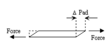
- Deflection of Elastomeric Bearing Pad

Pads
Where:
| = Longitudinal force to Bent , lbs | |
| = Total number of pads at Bent | |
| = Length of pad, in. | |
| = Width of pad, in. | |
| = Total thickness of elastomer layers for pad, in. | |
| = Shear Modulus, psi |
The shear modulus, G, varies with durometer, temperature, and time. To simulate this variance, the designer should run two sets of calculations, with G maximum and minimum. The values used shall be:
- = 150 psi
- = 300 psi
Column/pile deflections can be calculated from the following equation. Use Cols = 0 for non-flexible bents, i.e. semi-deep abutments or non-integral end bents.
- Column Deflection

Cols
Where:
| = Longitudinal force to Bent , lb | |
| = Bent height from point of fixity to top of beam, in. (*) | |
| = Gross moment of inertia of bent, , adjusted for skew | |
| = Column modulus of elasticity, psi (**) |
(*) For Pile Cap Intermediate Bents or Integral End Bents, use clear height plus Equivalent Cantilever Length defined in Seismic Design Section.
(**) To account for the composite material properties as well as the geometric properties of a C.I.P. pile, replace E with an equivalent modulus of elasticity, E', by solving the following equation, E'I = ESIS + ECIC. Where E' is the equivalent modulus of elasticity associated with the total moment of inertia, I.
Thus, the total deflection at bent is:
Pads+Cols
Step 2 – Convert Loads into terms of
- Since:
- Where:
- a, b, c, & d = known values from deflection equations
- And:
- Put in terms of :
Step 3 – Find Percentage of Wind Force to Each Bent
- Since:
- Then:
- Reduces to:
- Thus, is found by:
Once is known, the rest of the forces can then be calculated.
Note: Use the greater percentage calculated from the two different shear moduli, , for the substructure design.
751.2.4.7 Longitudinal Temperature Force Distribution
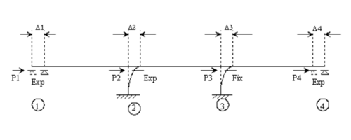
The longitudinal temperature forces applied to a continuous series of girders causes an incremental movement which deflects the supporting columns/piles and bearing pads. The amount each component deflects is dependant on the distance from the location the movement is being investigated to the point of thermal origin. Where the point of thermal origin is the location on the bridge where there is no thermal movement.
The deflection of each bent is calculated by the following equation:
Where:
| = the temperature movement at bent | |
| = coefficient of thermal expansion, | |
| = 0.000006 for concrete girders, | |
| = 0.0000065 for steel girders | |
| = length from thermal origin to bent | |
| = temperature fall, | |
| = temperature rise, |
The longitudinal forces applied at each bent can be determined by the following procedure.

- Support Deflections Due to Temperature Forces
Step 1 – Assume location of thermal origin
The location of the thermal origin may be assumed anywhere along the bridge. It is usually close to the middle of entire bridge length. The only care that must be taken is with the sign convention. As with the location of the thermal origin shown in figure above, the forces caused on the left side of the point of thermal origin must equal the forces on the right side of the thermal origin.
- Thus, for Figure above:
Step 2 – Calculate temperature movement at each bent in terms of distance “X”
| (in.) | |
Where:
| = the temperature movement from Bent 3 to the point of thermal origin (ft.) | |
| = Total deflection at Bent (in.) | |
| = span length | |
| = Bent number |
Step 3 – Calculate deflection computations at each bent in terms of force,
Deflections at each bent are caused by either the elastomeric bearing pads deflecting or the column/piles deflecting.
Bearing pad deflection is calculated from the following equation (Use Pads = 0 if there are no expansion pads).
- Deflection of Elastomeric Bearing Pad
Pads=
Where:
| = Longitudinal force to Bent , lbs | |
| = Total number of pads at Bent | |
| = Length of pad, in. | |
| = Width of pad, in. | |
| = Total thickness of elastomer layers for pad, in. | |
| = Shear Modulus, psi |
The shear modulus, , varies with durometer, temperature, and time. For 60 Durometer pads, use maximum associated with temperature fall, and minimum associated with temperature rise. The values used shall be:
- = 150 psi
- = 300 psi
Column/pile deflections can be calculated from the following equation. Use Cols = 0 for non-flexible bents, i.e. semi-deep abutments or non-integral end bents.
- Column Deflection
Cols=
Where:
| = Longitudinal force to Bent , lb. | |
| = Bent height from point of fixity to top of beam, in. (*) | |
| = Gross moment of inertia of bent, in.4, adjusted for skew | |
| = Column modulus of elasticity, psi (**) |
(*) For Pile Cap Intermediate Bents or Integral End Bents, use clear height plus Equivalent Cantilever Length defined in Seismic Design Section.
(**) To account for the composite material properties as well as the geometric properties of a C.I.P. pile, replace E with an equivalent modulus of elasticity, E', by solving the following equation, E'I = ESIS + ECIC. Where E' is the equivalent modulus of elasticity associated with the total moment of inertia, I.
Thus, the total deflection at bent , is:
Pads + Cols
Or for each individual bent:
Where:
, , , , & = known values from deflection equations
Step 4 – Set thermal deflection in terms of equal to the deflection in terms of for the corresponding bent numbers
Once the terms are combined in one equation, solve each bent equation for the corresponding bent force .
Where:
Step 5 - Solve for
- Since:
Substitue equations from Step 4 into the above equation and solve for .
Step 6 – Calculate forces
Once the variable is calculated, the values for each temperature force applied to the bents can be found. Two runs shall be done to account for for both “temperature rise” and “temperature fall”. The maximum load found between the two cases shall be used in design.