751.9 Bridge Seismic Design
751.9.1 Seismic Analysis and Design Specifications
All new or replacement bridges on the state system shall include seismic design and/or detailing to resist an expected seismic event per the Bridge Seismic Design Flowchart. For example, for a bridge in Seismic Design Categories A, B, C or D, complete seismic analysis or seismic detailing only may be determined as per “Bridge Seismic Design Flowchart”.
Preliminary Seismic Design Map: Preliminary seismic regions are shown with major routes and 1st and 2nd priority earthquake emergency routes. Seismic regions are preliminary since they are based on the assumption of Site Class D. The map uses the 2023 AASHTO Guide Specifications for LRFD Seismic Bridge Design (SGS), 3rd Ed. (Risk-targeted design spectra from USGS 2018 National seismic hazard model, NSHMP Static Data Services (usgs.gov)). Bold green lines are major routes. Orange highlighted roads are 1st or 2nd priority earthquake emergency routes. For additional information, See SEG 24-01.

Missouri is divided into four Seismic Design Categories. Most of the state is SDC A which requires minimal seismic design and/or detailing in accordance with SGS (Seismic Zone 1 of LRFD) and “Bridge Seismic Design Flowchart”. The other seismic design categories will require a greater amount of seismic design and/or detailing.
For seismic detailing only:
When AS is greater than 0.75 then use AS = 0.75 for abutment design where required per “Bridge Seismic Design Flowchart” and SEG 24-01
For complete seismic analysis:
When AS is greater than 0.75 then use AS = 0.75 at zero second for seismic analysis and response spectrum curve. See Example 1_SDC_Response_Spectra. The other data points on the response spectrum curve shall not be modified.
When existing bridges are identified as needing repairs or maintenance, a decision on whether to include seismic retrofitting in the scope of the project shall be determined per the “Bridge Seismic Retrofit Flowchart”, the extent of the rehabilitation work and the expected life of the bridge after the work. For example, if the bridge needs painting or deck patching, no retrofitting is recommended. However, redecking or widening the bridge indicates that MoDOT is planning to keep the bridge in the state system with an expected life of at least 30 more years. In these instances, the project core team should consider cost effective methods of retrofitting the existing bridge. Superstructure replacement requires a good substructure and the core team shall decide whether there is sufficient seismic capacity. Follow the design procedures for new or replacement bridges in forming logical comparisons and assessing risk in a rational determination of the scope of a superstructure replacement project specific to the substructure. For example, based on SPC and route, retrofit of the substructure could include seismic detailing only or a complete seismic analysis may be required determine sufficient seismic capacity. Economic analysis should be considered as part of the decision to re-use and retrofit, or re-build. Where practical, make end bents integral and eliminate expansion joints. Seismic isolation systems shall conform to AASHTO Guide Specifications for Seismic Isolation Design 4th Ed. 2023.
Bridge seismic retrofit for widenings shall be in accordance with Bridge Seismic Retrofit Flowchart. Seismic details should only be considered for widenings where they can be practically implemented and where they can be uniformly implemented as not to create significant stress redistribution in the structure. When a complete seismic analysis is required for widenings the existing structure shall be retrofitted and the new structural elements shall be detailed to resist seismic demand.
- Seismic Details for Widening (one side): When widening the bridge in one direction there is not a significant benefit, and it could be detrimental, to strengthen a new wing or column while ignoring the existing structure. It may be practical to use FRP wrap to retrofit the existing columns to provide a similar level of service to a new column with seismic details, but this will likely require design computations to verify (see below). For SDC C and D, seismic details typically require a T-joint detail in the beam cap and footing, but t-joint details shall be ignored if the existing beam cap is not retrofitted. For abutments it is not practical to dig up an existing wing solely to match the new wing design so the abutment need not be designed for mass inertial forces. SPM, SLE or owner’s representative approval is required to determine the appropriate level of seismic detail implementation.
- Seismic Details for Widening (both sides): When widening in both directions the wings shall be designed to resist the mass inertial forces. Seismic details shall be added to the new columns in SDC B only if the existing columns can be retrofitted with FRP wrap to provide a similar level of service as discussed below. SDC C and D bridges may be detailed and retrofitted similar to SDC B since retrofitting the beam cap or footing is likely not practical.
- Seismic Details for Widening (FRP wrap): Carbon or glass fiber reinforced polymer (FRP) composite wrap should be considered to strengthen the factored axial resistance of existing columns. There are limitations to the existing and achievable column factored axial resistance with FRP wrap. The goal of the FRP wrap is to increase the factored axial resistance of the existing column to be not less than the factored axial resistance of the new column with seismic details. If an existing column cannot be retrofitted with FRP wrap to match the factored axial resistance of a new column with seismic details at the same bent then seismic details shall be ignored for all columns in the bridge substructure. See AASHTO Guide Spec for Design of Bonded FRP Systems for Repair and Strengthening of Concrete Bridge Elements, March 2023, 2nd Ed., Appendix A, Example 6 for an example for increasing column factored axial resistance with FRP wrap. Use EPG 751.50 Standard Detailing Notes I5 on plans to report factored axial resistance of existing column and new column. The flexural resistance of the column is also increased with FRP wrap, but it may not be practical to match the flexural resistance of a new column using existing longitudinal steel. For additional references, see EPG 751.40.3.2 Bent Cap Shear Strengthening using FRP Wrap.
751.9.1.1 Applicability of Guidelines and Seismic Design Philosophy
SGS 3.1, 3.2, LRFD 3.4 and LRFD C3.4.1
EPG 751.9 supplements the above documentation for typical bridges in accordance with SGS 3.1. It does not apply to movable bridges, bridges with spans greater than 500 ft., suspension bridges, cable-stayed bridges, truss bridges or arch-type bridges. The State Bridge Engineer shall specify and/or approve appropriate provisions or specifications for non typical bridges. There are special considerations for single-span bridges, temporary bridges and bridges with stage construction.
Critical and Recovery Bridges are not specifically addressed in SGS specification, SGS 3.1. Operational classification shall be in accordance with SGS 3.1 and SGS 3.2. Bridges shall be designed for the life safety performance objective using at a minimum the limit state of incipient collapse or unacceptable performance for geotechnical failure modes at a targeted risk of approximately 1.5 percent over 75 years in accordance with SGS 3.2 Higher levels of performance, such as the operational objective, may be established and authorized by the bridge owner. Critical and Recovery bridges shall be designed in accordance with AASHTO Guidelines for Performance-Based Seismic Design of Highway Bridges, 1st ed.
The following categories are used throughout EPG:
- Nonseismic = Bridges requiring a static design only. Minimal seismic details in accordance with SDC A are still required.
- Seismic Details = This category refers to SDC A (SD1 ≥ 0.1), B, C and D bridges that do not require a seismic design, but do require higher levels of seismic detailing.
- Complete Seismic Analysis = Bridges requiring a full seismic analysis. SDC C or D bridges may be applicable based on the importance of the route.
Life safety for the design event shall be taken to imply that the bridge has a low probability of collapse but may suffer significant damage, and significant disruption to service is possible. Partial or complete replacement may be required in accordance with SGS 3.2. Hazard to human life should be minimized, and essential bridges should continue to function after an earthquake. Bridges are designed for good ductility and displacement control and are allowed to suffer minor, acceptable damage in order to prevent major, unacceptable damage.
Note: For seismic design force concepts and guidance, follow the seismic design process (EPG 751.9.1.3 thru 751.9.4) and modify design/details of LFD as necessary to meet SGS and LRFD seismic requirements until LRFD seismic section is created (modified EPG 751.9.1.3 thru 751.9.4).
All new or replacement bridges on the state system shall include seismic design and/or detailing to resist an expected seismic event (seismic design category) per the Bridge Seismic Design Flowchart.
- For a major bridge, the State Bridge Engineer will decide the design as a life safety or critical/essential or recovery bridge in accordance with SGS 3.1, SGS 3.2 and SGS C3.2.
- Except for section 7 of the AASHTO Guide Specifications for LRFD Seismic Bridge Design (SGS) is based on Displacement Based Design. The AASHTO LRFD Bridge Design Specifications (LRFD) is based on Force Based Design. For seismic details and design concept use the SGS when information is available otherwise use LRFD. Seismic analysis shall be performed using displacement-based design (for exception see SGS 7).
| Seismic Design Category/Seismic Zone by Code | ||
|---|---|---|
| Value of design spectral acceleration coefficient at 1.0 second period, SD1 SGS 3.4.1 and 3.5 |
1AASHTO Guide Specifications for LRFD Seismic Bridge Design (SGS) SGS table 3.5-1 Seismic Design Category (SDC) |
2AASHTO LRFD Bridge Design Specifications (LRFD) LRFD Table 3.10.6-1 Seismic Zones |
| SD1 < 0.10 | A1 | 1 |
| 0.10 ≤ SD1 < 0.15 | A23 | 13 |
| 0.15 ≤ SD1 < 0.30 | B | 2 |
| 0.30 ≤ SD1 < 0.50 | C | 3 |
| 0.50 ≤ SD1 | D | 4 |
1SGS is required for seismic design. LRFD is shown because SGS refers to LRFD for support, and understanding the equivalency category and zone may be important. In accordance with SGS, all bridge designs must meet the requirements for SDC A (Seismic Zone 1). Additional seismic details are typically required for higher seismic design categories.
2LRFD inequalities are different. Use SGS as shown.
3Structural member shall be detailed in accordance with SDC B (SGS 8.2) if bridge carry a 1st or 2nd priority earthquake emergency route.
751.9.1.2 LRFD Seismic Details
751.9.1.2.1 Seismic Details for Column Supported on Footing
| Seismic Design Category, SDC B | |||||||||||
|---|---|---|---|---|---|---|---|---|---|---|---|
| Shear Reinf. |
Diameter (inch) |
Min. cover (inch) |
Core D' (inch) |
spiral/hoop size1 | Area of spiral/hoop bar Asp (sq. inch) |
Pitch or space s (inch) |
f'c (ksi) |
Ro = 4Asp/(D'*s) SGS Eq 8.6.2‐7 |
Ro min SGS 8.6.5 |
||
| Spiral | 36 | 1.5 | 32.375 | 5 | 0.307 | 4 | 3 | 0.0095 | ≥ | 0.003 | OK |
| Spiral | 42 | 1.5 | 38.375 | 5 | 0.307 | 4 | 3 | 0.0080 | ≥ | 0.003 | OK |
| Spiral | 48 | 1.5 | 44.375 | 5 | 0.307 | 4 | 3 | 0.0069 | ≥ | 0.003 | OK |
| Spiral | 54 | 1.5 | 50.375 | 5 | 0.307 | 4 | 3 | 0.0061 | ≥ | 0.003 | OK |
| Hoop | 60 | 1.5 | 56.375 | 5 | 0.307 | 4 | 3 | 0.0054 | ≥ | 0.003 | OK |
| Hoop | 66 | 1.5 | 62.375 | 5 | 0.307 | 4 | 3 | 0.0049 | ≥ | 0.003 | OK |
| Hoop | 72 | 1.5 | 68.375 | 5 | 0.307 | 4 | 3 | 0.0045 | ≥ | 0.003 | OK |
| Seismic Design Category, SDC C and D | |||||||||||
|---|---|---|---|---|---|---|---|---|---|---|---|
| Shear Reinf. |
Diameter (inch) |
Min. cover (inch) |
Core D' (inch) |
spiral/hoop size1 | Area of spiral/hoop bar Asp (sq. inch) |
Pitch or space s (inch) |
f'c (ksi) |
Ro = 4Asp/(D'*s) SGS Eq 8.6.2‐7 |
Ro min SGS 8.6.5 |
||
| Spiral | 36 | 1.5 | 32.375 | 5 | 0.307 | 4 | 3 | 0.0095 | ≥ | 0.005 | OK |
| Spiral | 42 | 1.5 | 38.375 | 5 | 0.307 | 4 | 3 | 0.0080 | ≥ | 0.005 | OK |
| Spiral | 48 | 1.5 | 44.375 | 5 | 0.307 | 4 | 3 | 0.0069 | ≥ | 0.005 | OK |
| Spiral | 54 | 1.5 | 50.375 | 5 | 0.307 | 4 | 3 | 0.0061 | ≥ | 0.005 | OK |
| Hoop | 60 | 1.5 | 56.375 | 5 | 0.307 | 4 | 3 | 0.0054 | ≥ | 0.005 | OK |
| Hoop | 66 | 1.5 | 62.25 | 6 | 0.442 | 4 | 3 | 0.0071 | ≥ | 0.005 | OK |
| Hoop | 72 | 1.5 | 68.25 | 6 | 0.442 | 4 | 3 | 0.0065 | ≥ | 0.005 | OK |
| Note: | 1For simplification use minimum #5 spiral/hoop bar. | SGS 8.8.9 |
| Ro shall be ≥ 0.003 in SDC B and 0.005 in SDC C and D. No need to meet LRFD 5.6.4.6‐1 & 5.11.4.1.4‐1 minimum Ro requirements. | SGS 8.6.5 | |
| Use 4" spiral pitch/hoop spacing for column to meet long. bar splice area requirements. | LRFD 5.11.4.1.6 | |
| Use spiral or hoop but combination of spiral reinforcement with hoops shall not be used except in the footing or bent cap. | SGS 8.8.7 | |
| Closed tie (Hoop) shall use 135‐degree hook with an extension of 6 bar diameters but not less than 3". | SGS 8.8.9 | |
| Welding of reinforcing steel (spiral, hoop and longitudinal) is not permitted due to the prohibitive cost of weld inspection. | ||
| Spiral does not need to meet end tail requirements of SGS 8.8.7. | ||
| (1) Anchorage of spiral reinforcement shall be provided by 1 1/2 extra turns of spiral reinforcement at end of the spiral unit. | ||
| (2) Lac = max(Lac from SGS 8.8.4, 1.25 Ld) or Ldh, but shall be extended to the clear cover specified herein. | ||
| (3) 11 inches for #8 thru #11 bars and 14 inches for #14 bars. | ||
| (4) Plastic hinge area for SDC B: Lpr ≥ max(1.0 * col dia, 1/6 clear col ht., 18") | SGS C8.8.9 & LRFD C5.11.4.1.4 | |
| (4) Plastic hinge area for SDC C and D: Lpr ≥ max(1.5 * col dia, Lp, 1/6 clear column ht.) | SGS 4.11.6 and 4.11.7 | |
| (4) Long reinf. and spiral bar shall not be spliced in plastic hinge area. If splice is unavoidable, a mechanical bar splice shall be used. | SGS 8.8.3 LRFD 5.11.4.1.6 | |
| (5) Minimum lap: Use greater of EPG 751.5.9.2.8.2 Class B lap splice or 60 bar diameters. Lap splices and mechanical bar splices are to be alternately staggered at least 24”at two different locations. | LRFD 5.10.8.4.3b | |
| For dowel bar in beam cap, See EPG 751 .22.2.7 Dowel Bars | ||
| For additional requirements of column joints in SDC C and D, See EPG 751 .9.1.2.4 T-Joint (Column Joint) Connections for Seismic Design Category C and D. | ||
| Use Figure 751.9.1.2.1.1 and Figure 751.9.1.2.1.2 for seismic detail option. For complete seismic design option spiral/hoop bar size shall be increased up to #6 and pitch/spacing shall be reduced as needed by design. Absolute minimum clearance is 1.5 inches. |
-
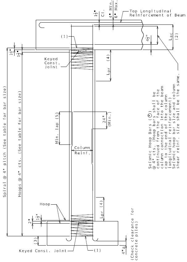 Figure 751.9.1.2.1.1 Seismic Details for Column Supported on Footing

-
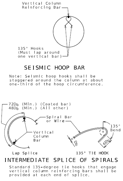 Figure 751.9.1.2.1.2 Seismic Bar Details

751.9.1.2.2 Seismic Details for Non-oversized Drilled Shaft
| Seismic Design Category, SDC B | ||||||||||||
|---|---|---|---|---|---|---|---|---|---|---|---|---|
| Shear Reinf. |
Diameter (inch) |
Min. cover (inch) |
Core D' (inch) |
spiral/hoop size1 | 1 for single bar 2 for bundle hoop bars |
Area of spiral/hoop bar Asp (sq. inch) |
Pitch or space s (inch) |
f'c (ksi) |
Ro = 4Asp/(D'*s) SGS Eq 8.6.2‐7 |
Ro min SGS 8.6.5 |
||
| Spiral | 36 | 6 | 23.375 | 5 | 1 | 0.307 | 6 | 4 | 0.0087 | ≥ | 0.003 | OK |
| Spiral | 42 | 6 | 29.375 | 5 | 1 | 0.307 | 6 | 4 | 0.0070 | ≥ | 0.003 | OK |
| Spiral | 48 | 6 | 35.375 | 5 | 1 | 0.307 | 6 | 4 | 0.0058 | ≥ | 0.003 | OK |
| Spiral | 54 | 6 | 41.375 | 5 | 1 | 0.307 | 6 | 4 | 0.0049 | ≥ | 0.003 | OK |
| Spiral | 60 | 6 | 47.375 | 5 | 1 | 0.307 | 6 | 4 | 0.0043 | ≥ | 0.003 | OK |
| Hoop | 66 | 6 | 53.375 | 5 | 1 | 0.307 | 6 | 4 | 0.0038 | ≥ | 0.003 | OK |
| Hoop | 72 | 6 | 59.375 | 5 | 1 | 0.307 | 6 | 4 | 0.0034 | ≥ | 0.003 | OK |
| Hoop | 78 | 6 | 65.25 | 6 | 1 | 0.442 | 6 | 4 | 0.0045 | ≥ | 0.003 | OK |
| Seismic Design Category, SDC C and D | ||||||||||||
|---|---|---|---|---|---|---|---|---|---|---|---|---|
| Shear Reinf. |
Diameter (inch) |
Min. cover (inch) |
Core D' (inch) |
spiral/hoop size1 | 1 for single bar 2 for bundle hoop bars |
Area of spiral/hoop bar Asp (sq. inch) |
Pitch or space s (inch) |
f'c (ksi) |
Ro = 4Asp/(D'*s) SGS Eq 8.6.2‐7 |
Ro min SGS 8.6.5 |
||
| Spiral | 36 | 6 | 23.375 | 5 | 1 | 0.307 | 6 | 4 | 0.0087 | ≥ | 0.005 | OK |
| Spiral | 42 | 6 | 29.375 | 5 | 1 | 0.307 | 6 | 4 | 0.0070 | ≥ | 0.005 | OK |
| Spiral | 48 | 6 | 35.375 | 5 | 1 | 0.307 | 6 | 4 | 0.0058 | ≥ | 0.005 | OK |
| Spiral | 54 | 6 | 41.25 | 6 | 1 | 0.442 | 6 | 4 | 0.0071 | ≥ | 0.005 | OK |
| Spiral | 60 | 6 | 47.25 | 6 | 1 | 0.442 | 6 | 4 | 0.0062 | ≥ | 0.005 | OK |
| Hoop | 66 | 6 | 53.25 | 6 | 1 | 0.442 | 6 | 4 | 0.0055 | ≥ | 0.005 | OK |
| Hoop | 72 | 6 | 59.375 | 5 | 2 | 0.614 | 8 | 4 | 0.0052 | ≥ | 0.005 | OK |
| Hoop | 78 | 6 | 65.25 | 6 | 2 | 0.884 | 8 | 4 | 0.0068 | ≥ | 0.005 | OK |
| Note: | 1For simplification use minimum #5 spiral/hoop bar. | SGS 8.8.9 |
| Ro shall be ≥ 0.003 in SDC B and 0.005 in SDC C and D. No need to meet LRFD 5.6.4.6‐1 & 5.11.4.1.4‐1 minimum Ro requirements. | SGS 8.6.5 | |
| Closed tie (Hoop) shall use 135‐degree hook with an extension of 6 bar diameters but not less than 3". | SGS 8.8.9 | |
| Spiral does not need to meet end tail requirements of SGS 8.8.7. | ||
| For (2) and (4), see EPG 751.9.1.2.1 Seismic Details for Column Supported on Footing. | ||
| (6) Anchorage of spiral reinforcement shall be provided by 1 1/2 extra turns of spiral reinforcement at end of the spiral unit. | ||
| (7) Plastic hinge area for SDC B: Lpr ≥ drilled shaft diameter. | SGS C8.8.9 and LRFD C5.11.4.1.4 | |
| (7) Plastic hinge area for SDC C and D: Lpr ≥ max(1.5 * Column dia., Lp, drilled shaft diameter). | SGS 4.11.6 and 4.11.7 | |
| (7,8) Long reinforcement and spiral bar shall not be spliced in plastic hinge area. If splice is unavoidable, a mechanical bar splice shall be used. | SGS 8.8.3 and LRFD 5.11.4.1.6 | |
| (8) Plastic hinge area : Lpr ≥ drilled shaft diameter. | ||
| (9) Minimum lap: Use greater of EPG 751.5.9.2.8.2 Class B lap splice or 60 bar diameters. Lap splices and mechanical bar splices are to be alternately staggered at least 24”at two different locations. | LRFD 5.10.8.4.3b | |
| (10) Use spiral or hoop but combination of spiral reinforcement with hoops shall not be used except in the bent cap. From above table if hoop required for drilled shaft than hoop shall be used in the column and if spiral required for drilled shaft than spiral shall be used in column. Use spiral or hoop bar size and pitch or spacing per EPG 751.9.1.2.1 | SGS 8.8.7 | |
| Welding of reinforcing steel (spiral, hoop and longitudinal) is not permitted due to the prohibitive cost of weld inspection. | ||
| For detail simplification consider drilled shaft 6” larger than column. Avoid sizing shafts 12” larger than column. | ||
| For column and beam detail requirements, see EPG 751.9.1.2.1. | ||
| For oversized shaft (generally 18" minimum larger than column), see EPG 751.9.1.2.3 Seismic Details for Oversized Drilled Shaft. | ||
| For additional requirements of column joints in SDC C and D, See EPG 751.9.1.2.4 T-Joint (Column Joint) Connections for Seismic Design Category C and D. | ||
| Use Figure 751.9.1.2.2 for seismic detail option. For complete seismic design option spiral/hoop bar size shall be increased up to #6 and pitch/spacing shall be 6” by design. Absolute minimum clearance is 5 inches. If #6 at 6” spiral or hoop do not meet design requirements, then use 2-#6 hoop bars @ 8” spacing. | ||
| For seismic bar details (spiral and hoop), see Figure 751.9.1.2.1.2 |
-
 Figure 751.9.1.2.2 Seismic Details for Non-oversized Drilled Shaft

751.9.1.2.3 Seismic Details for Oversized Drilled Shaft
| Seismic Design Category, SDC B | ||||||||||||
|---|---|---|---|---|---|---|---|---|---|---|---|---|
| Shear Reinf. |
Diameter (inch) |
Min. cover (inch) |
Core D' (inch) |
spiral/hoop size1 | 1 for single bar 2 for bundle hoop bars |
Area of spiral/hoop bar Asp (sq. inch) |
Pitch or space s (inch) |
f'c (ksi) |
Ro = 4Asp/(D'*s) SGS Eq 8.6.2‐7 |
Ro min SGS 8.6.5 |
||
| Spiral | 36 | 6 | 23.375 | 5 | 1 | 0.307 | 6 | 4 | 0.0087 | ≥ | 0.003 | OK |
| Spiral | 42 | 6 | 29.375 | 5 | 1 | 0.307 | 6 | 4 | 0.0070 | ≥ | 0.003 | OK |
| Spiral | 48 | 6 | 35.375 | 5 | 1 | 0.307 | 6 | 4 | 0.0058 | ≥ | 0.003 | OK |
| Spiral | 54 | 6 | 41.375 | 5 | 1 | 0.307 | 6 | 4 | 0.0049 | ≥ | 0.003 | OK |
| Spiral | 60 | 6 | 47.375 | 5 | 1 | 0.307 | 6 | 4 | 0.0043 | ≥ | 0.003 | OK |
| Spiral/Hoop | 66 | 6 | 53.375 | 5 | 1 | 0.307 | 6 | 4 | 0.0038 | ≥ | 0.003 | OK |
| Spiral/Hoop | 72 | 6 | 59.375 | 5 | 1 | 0.307 | 6 | 4 | 0.0034 | ≥ | 0.003 | OK |
| Spiral/Hoop | 78 | 6 | 65.25 | 6 | 1 | 0.442 | 6 | 4 | 0.0045 | ≥ | 0.003 | OK |
| Seismic Design Category, SDC C and D | ||||||||||||
|---|---|---|---|---|---|---|---|---|---|---|---|---|
| Shear Reinf. |
Diameter (inch) |
Min. cover (inch) |
Core D' (inch) |
spiral/hoop size1 | 1 for single bar 2 for bundle hoop bars |
Area of spiral/hoop bar Asp (sq. inch) |
Pitch or space s (inch) |
f'c (ksi) |
Ro = 4Asp/(D'*s) SGS Eq 8.6.2‐7 |
Ro min SGS 8.6.5 |
||
| Spiral | 36 | 6 | 23.375 | 5 | 1 | 0.307 | 6 | 4 | 0.0087 | ≥ | 0.005 | OK |
| Spiral | 42 | 6 | 29.375 | 5 | 1 | 0.307 | 6 | 4 | 0.0070 | ≥ | 0.005 | OK |
| Spiral | 48 | 6 | 35.375 | 5 | 1 | 0.307 | 6 | 4 | 0.0058 | ≥ | 0.005 | OK |
| Spiral | 54 | 6 | 41.25 | 6 | 1 | 0.442 | 6 | 4 | 0.0071 | ≥ | 0.005 | OK |
| Spiral | 60 | 6 | 47.25 | 6 | 1 | 0.442 | 6 | 4 | 0.0062 | ≥ | 0.005 | OK |
| Spiral/Hoop | 66 | 6 | 53.25 | 6 | 1 | 0.442 | 6 | 4 | 0.0055 | ≥ | 0.005 | OK |
| Hoop | 72 | 6 | 59.375 | 5 | 2 | 0.614 | 8 | 4 | 0.0052 | ≥ | 0.005 | OK |
| Hoop | 78 | 6 | 65.25 | 6 | 2 | 0.884 | 8 | 4 | 0.0068 | ≥ | 0.005 | OK |
| Note: | 1For simplification use minimum #5 spiral/hoop bar. | SGS 8.8.9 |
| Ro shall be ≥ 0.003 in SDC B and 0.005 in SDC C and D. No need to meet LRFD 5.6.4.6‐1 & 5.11.4.1.4‐1 minimum Ro requirements. | SGS 8.6.5 | |
| Closed tie (Hoop) shall use 135‐degree hook with an extension of 6 bar diameters but not less than 3". | SGS 8.8.9 | |
| Spiral does not need to meet end tail requirements of SGS 8.8.7. | ||
| For (2) and (4), see EPG 751.9.1.2.1 Seismic Details for Column Supported on Footing. | ||
| (11) Anchorage of spiral reinforcement shall be provided by 1 1/2 extra turns of spiral reinforcement at end of the spiral unit. | ||
| (12) Plastic hinge area for SDC B: Lpr ≥ drilled shaft diameter. | SGS C8.8.9 and LRFD C5.11.4.1.4 | |
| (12) Plastic hinge area for SDC C and D: Lpr ≥ max(1.5 * Column dia., Lp, drilled shaft diameter). | SGS 4.11.6 and 4.11.7 | |
| (12) Long reinforcement and spiral bar shall not be spliced in plastic hinge area. If splice is unavoidable, a mechanical bar splice shall be used. | SGS 8.8.3 and LRFD 5.11.4.1.6 | |
| (13) Plastic hinge area : Lpr ≥ drilled shaft diameter. | ||
| (14) Minimum lap: Use greater of EPG 751.5.9.2.8.2 Class B lap splice or 60 bar diameters. Lap splices and mechanical bar splices are to be alternately staggered at least 24”at two different locations. | LRFD 5.10.8.4.3b | |
| (15) Since column reinforcement embedded into drilled shaft, clear spacing between column reinforcement shall be 5” min. | ||
| (16) Spiral pitch or hoop bar spacing shall be same as drilled shaft requirements. | ||
| Use spiral or hoop but combination of spiral reinforcement with hoops shall not be used in a reinforcement cage except in bent cap. Spirals in the column cage and hoops in the drilled shaft cage can be used for oversized drilled shaft | SGS 8.8.7 | |
| Welding of reinforcing steel (spiral, hoop and longitudinal) is not permitted due to the prohibitive cost of weld inspection. | ||
| Hoops are preferred for drilled shafts with diameters at least 2’-6” larger than column. Spirals shall be used in drilled shafts that are oversized by 18” or 24” due to potential interference between the hooks and the column reinforcing cage. | ||
| Column confinement: | ||
| For column use spiral/pitch or hoop/spacing and bar size per column shear reinforcement requirements. | ||
| Drilled shaft confinement: | ||
| Exterior cage: From above table use spiral/pitch or hoop/spacing for drilled shaft. | ||
| Interior cage: Column confinement reinforcement bar size from column shear reinforcement table shall be spaced or pitched same as drilled shaft and provided over entire embedded length of column steel in drilled shaft. |
||
| For column and beam detail requirements, see column shear reinforcement. | ||
| For additional requirements of column joints in SDC C and D, See EPG 751.9.1.2.4 T-Joint (Column Joint) Connections for Seismic Design Category C and D. | ||
| Use Figure 751.9.1.2.3 for seismic detail option. For complete seismic design option spiral/hoop bar size shall be increased up to #6 and pitch/spacing shall be 6” by design. Absolute minimum clearance is 5 inches. If #6 at 6” spiral or hoop do not meet design requirements, then use 2-#6 hoop bars @ 8” spacing. | ||
| For seismic bar details (spiral and hoop), see Figure 751.9.1.2.1.2 |
-
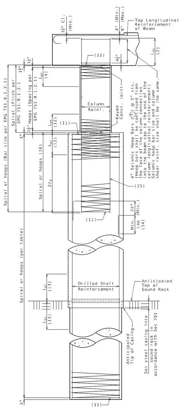 Figure 751.9.1.2.3 Seismic Details for Oversized Drilled Shaft

751.9.1.2.4 T-Joint (Column Joint) Connections for Seismic Design category C and D
Minimum joint reinforcement shall be provided as shown below. Reinforcement marked as “additional” shall not be used to satisfy other load requirements.
751.9.1.2.4.1 Bent Cap Joint Shear Reinforcement
| 1. | Additional Vertical Stirrups Outside the Joint Region | SGS 8.13.5.1.1 |
| Where, | ||
| Total area of column longitudinal reinforcement anchored in the joint | ||
| Minimum total area of additional vertical stirrups on each side of joint | ||
| Total area of vertical stirrups shall be provided transversely within a distance equal to the column diameter extending from each face of the column as shown in Figure 751.9.1.2.4.1a. For additional vertical stirrups size and spacing limitations, see EPG 751.31.3.1. | ||
| 2. | Additional Vertical Stirrups Inside the Joint Region | SGS 8.13.5.1.2 |
| Where, | ||
| Total area of column longitudinal reinforcement anchored in the joint | ||
| Minimum total area of vertical stirrups inside the joint region | ||
| Total area of vertical stirrups spaced evenly over the column inside the joint region as shown in Figure 751.9.1.2.4.1a. For additional vertical stirrups size and spacing limitations, see EPG 751.31.3.1. | ||
| 3. | Additional Longitudinal Cap Beam Reinforcement | SGS 8.13.5.1.3 |
| Where, | ||
| Total area of column longitudinal reinforcement anchored in the joint | ||
| Minimum total area of additional longitudinal reinforcement in top and bottom faces of the cap beam | ||
| The additional longitudinal reinforcement shall be extended at least one column diameter plus development length from face of the column as shown in Figure 751.9.1.2.4.1a | ||
| 4. | Horizontal J-Bars | SGS 8.13.5.1.4 |
| #4 Horizontal J-bars shall be hooked around the longitudinal reinforcement on each face of the cap beam at every other stirrup inside the joint as shown in Figure 751.9.1.2.4.1b. | ||
| When complete seismic analysis is required per Bridge Seismic Design Flowchart, joint shear reinforcement shall be provided in accordance with AASHTO Guide Specifications for LRFD Seismic Bridge Design (SGS). Modify above information and provide additional reinforcement as needed by design. | SGS 8.12 and 8.13 | |
-
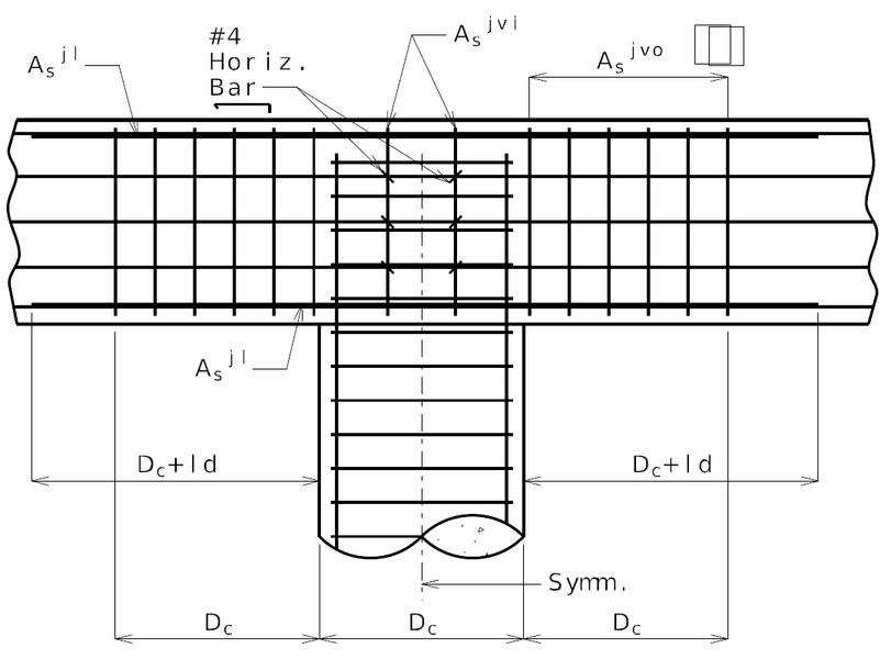 Figure 751.9.1.2.4.1a Elevation Showing Column and Beam Cap Reinforcement
(SDC C and D only)

-
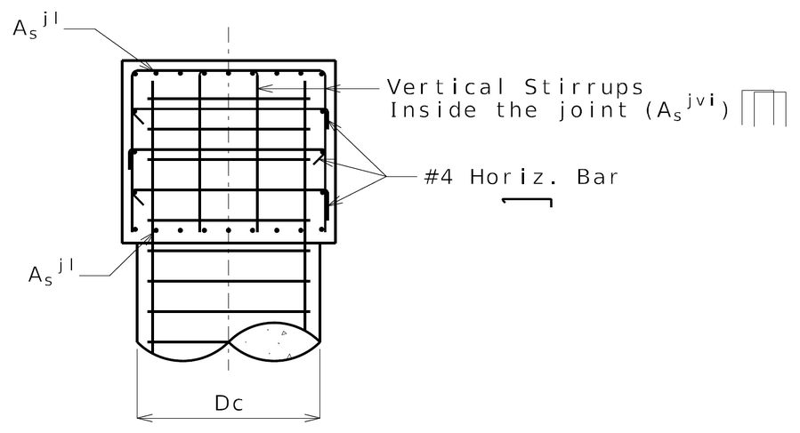 Figure 751.9.1.2.4.1b Section Showing Column and Beam Cap Reinforcement
(SDC C and D only)

751.9.1.2.4.2 Footing (Spread Footing and Pile Footing) Joint Shear Reinforcement
| For seismic detail option, use following information for spread footing and pile footing | SGS 6.4.7 | ||
| Vertical shear reinforcement #5 at about 12” each way shall be placed around the column perimeter within a horizontal dimension from face of the column equal to minimum as shown in Figure 751.9.1.2.4.2a and Figure 751.9.1.2.4.2b. #6 maximum bar size shall be used for vertical shear reinforcement. | |||
| Effective depth from top of footing to lower reinforcement mat. | |||
| Additional longitudinal horizontal reinforcement at top of footing, : | |||
| = | |||
| Where, | |||
| = Total area of column longitudinal reinforcement anchored in the joint | |||
| = Expected yield stress of column longitudinal reinforcement | |||
| = 68 ksi for ASTM A706 and ASTM A615 | SGS Table 8.4.2-1 | ||
| = Minimum yield stress of column longitudinal reinforcement | |||
| = 60 ksi for ASTM A706 and ASTM A615 | SGS Table 8.4.2-1 | ||
| The additional longitudinal reinforcement shall be extended at least up to a distance plus development length from face of the column and must be placed so that the reinforcement goes through the column reinforcement as shown in Figure 751.9.1.2.4.2a and Figure 751.9.1.2.4.2b shall be provided in both directions in the footing. | |||
| When complete seismic analysis is required per Bridge Seismic Design Flowchart, joint shear reinforcement shall be provided in accordance with AASHTO Guide Specifications for LRFD Seismic Bridge Design (SGS). Modify above information and provide additional reinforcement as needed by design. | SGS 6.4.5, 6.4.6 and 6.4.7 | ||
-
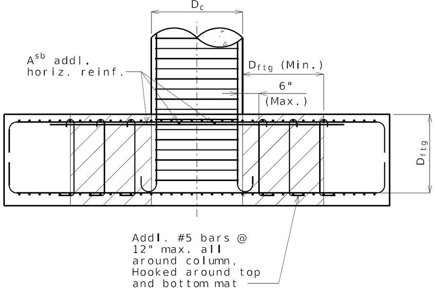 Figure 751.9.1.2.4.2a Spread Footing Joint Shear Reinforcement

-
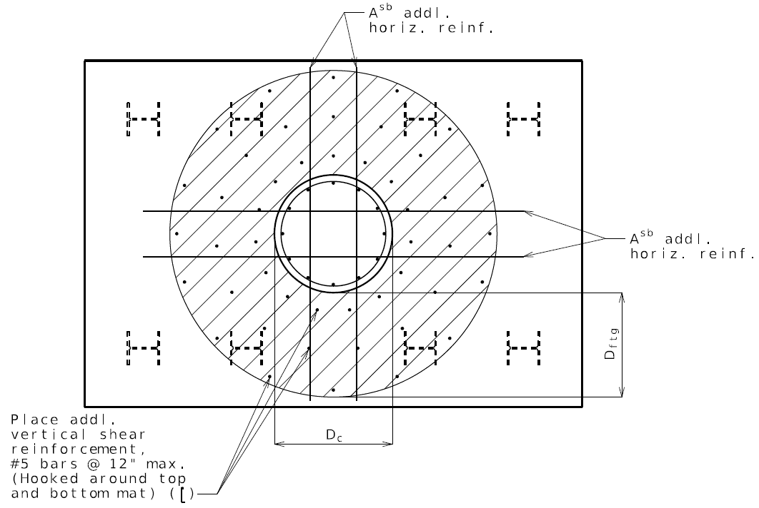 Figure 751.9.1.2.4.2b Pile Footing Joint Shear Reinforcement

751.9.1.3 Seismic Design Force Concepts
As shown in Fig. 751.9.1.3.1(a), a two span bridge can be modeled as a single–degree-of-freedom lumped-mass system (Fig. 751.9.1.3.1(b)). For a single degree-of-freedom lumped-mass system, the total elastic seismic design force is equal to
- F = m x cs x g
where:
- m is the total structural mass
- cs is the elastic seismic response coefficient
- g is the gravitational acceleration constant
The elastic seismic response coefficient is given by the dimensionless formula
| AASHTO Div. I-A, Equation 3-1 |
where:
- A = the acceleration coefficient on rock from AASHTO Division I-A, Article 3.2; the acceleration coefficients for Missouri are shown in Fig. 751.9.1.3.3.
- S = the dimensionless coefficient for the soil profile characteristics of the site as given in Article 3.5. S = 1.0, 1.2, 1.5, and 2.0 for soil profile type I, II, III, and IV respectively.
- T = the fundamental period of the bridge,
- where: k is the structural lateral stiffness
- m is the structural mass

The elastic design acceleration spectra shown in Fig. 751.9.1.3.2 is a plot of structural period T versus the maximum acceleration quantity of the structure. For example: a bridge with the foundation period T1 is subjected to an earthquake having a rock acceleration of . The maximum acceleration of this bridge during the whole seismic excitation will be (see Fig. 751.9.1.3.2).

From Fig. 751.9.1.3.1, it can be seen that the acceleration of soil is larger than the acceleration of rock by an amplification factor S. Soil type is important to the evaluation of ground acceleration. From Figs. 751.9.1.3.1 and 751.9.1.3.2, stated briefly, the design acceleration spectrum is a plot of the maximum acceleration to a specified seismic load for all possible single degree-offreedom systems.
Using the above mentioned concept, AASHTO considers four analysis procedures to calculate elastic earthquake design force for the Multiple Degree of Freedom (MDOF) System in order of increasing complexity. Theses are:
- Procedure 1 – Uniform Load Method
- Procedure 2 – Single-Mode Spectral Method
- Procedure 3 – Multi-Mode Spectral Method
- Procedure 4 – Time History Method
MoDOT practice is to use the Multi-Mode Method for all bridges, because the Uniform Load and Single-Mode Methods are inadequate for irregular bridges and the Time History Method requires an excessive level of numerical integration time and time history records being used. A seismic structural analysis program, such as SEISAB, performs a linear elastic multi-mode response spectrum analysis, accounting also for inertial effects, damping, and modal combination, and determines seismic forces and displacements at individual joints and members.
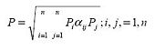
In the Multi-mode Spectral Method, the seismic deign force, P, of a specific structural component can be calculated by taking the square root of the sum of the squares (SRSS) or the complete quadratic combination (CQC) of the design for Pi corresponding to the ith mode of the structural component.
- SRSS approach:
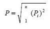
- SRSS approach:

- CQC approach:
- CQC approach:

- where:
- and
- where:
where n = the total number of modes of structure considered, Pi is calculated according to seismic design force Fi which is the design force corresponding to the structural ith mode with fundamental period of Ti and seismic response coefficient of Csi, Pi and Fi represent internal force of individual structural component and external seismic force applied to the structure respectively, Pj is similar to Pi , αij is the cross-correlation coefficient indicating the crosscorrelation between modes i and j, wi is the natural frequencies corresponding to the ith mode and ρ is the damping ratio (i.e. 0.05). For more detailed descriptions of procedures 1, 2, 3, and 4, see AASHTO Division I-A 4.3-4.6 and for a more detailed description of how to calculate Pi and Fi, see AASHTO Division I-A Commentary C.4.5.4.
For Seismic Performance Category (SPC) A, the above mentioned analysis procedure is not required.
For a regular bridge in SPC B, C, or D, procedure 1 and 2 are the minimum required analysis methods, procedure 3 is strongly recommended. A regular bridge, as described in AASHTO Division I-A, 4.2 has fewer than seven spans, no abrupt changes in weight, stiffness, or geometry and no large change in these parameters from span to span, or support to support (abutments excluded). Any bridge not satisfying the definition of a regular bridge is considered to be irregular. For an irregular bridge, procedure 3 must be used. The designer may use procedure 4 in place of procedure 3 if so desired.
Multi-mode spectral analysis is recommended for most bridges. Time History analysis is generally not recommended because its application requires considerable engineering judgement and experience.

Note: For LFD, use Fig. 751.9.1.3.3 Seismic Map to determine seismic performance categories (SPC A, B, C and D). For LRFD, use EPG Figure 751.9.1 Preliminary Seismic Design Map to determine preliminary seismic design category (SDC A (A1 and A2), B, C, and D) based on site class D.
751.9.1.4 Seismic Performance Category (SPC), Acceleration Coefficient (A)
| Additional Information |
| AASHTO Div. I-A, 3.2-3.4, and foldout map (Figure 1.5) at back of Division I-A |
Missouri is divided into four Seismic Performance Categories (SPC A, B, C and D, see Fig. 751.9.1.3.3, based on Acceleration Coefficients (A). The map for SPC and rock acceleration A is based on a 90% probability that the horizontal rock acceleration will not be exceeded in the 50-year lifetime of the bridge, corresponding to a return period of 475 years. For Missouri, the maximum A=0.36. For bridges with A > 0.29, an additional factor called Importance Classification (IC) is used to distinguish between SPC C and D.
751.9.1.5 Elastic and Plastic Design
| Additional Information |
| AASHTO Div. I-A, 3.7 |
In some cases, bridges can resist seismic forces elastically, that is, without permanent deformations. In other cases, it is not economical to design a bridge for elastic behavior under seismic loading, so the bridge may be designed for inelastic (plastic) behavior. However, plastic design requires careful detailing to ensure ductility and connections with higher energy absorption characteristics. Plastic behavior is nonlinear, but AASHTO Division I-A allows an approximate analysis procedure using a linear elastic analysis along with the application of a response modification factor (R) to account for the assumed level of ductility and redundancy. This allows the use of linear elastic analysis programs such as SEISAB (or any other seismic analysis program). Response modification factors are specified in AASHTO 1-A, Article 3.7. An example of ductility demand is described below:
| Additional Information |
| AASHTO Div. I-A, 1992 Commentary C3.6 |
- In an elastic seismic analysis, a column in a multiple-column bent is subjected to an elastic moment, Me , and a rotation, θmax at the bottom of the column. The dashed line in Figure 751.9.1.5 represents the elastic moment demand. If plastic behavior is allowed and a maximum ductility factor, μ, equal to 5 is used, then . The column is then sized so that its plastic moment capacity, Mp, is greater than or equal to the modified elastic moment, MME, such that . This is based on the assumption that the deformations produced by a given seismic input force, F, are essentially the same for both elastic column behavior and for column yielding behavior at a ductility demand of μ = 5. Response modification factors (R) are allowed because of component ductility capacity and because of redundancy provided by adjacent columns, piers, and abutments.

- rotation at bottom of column (elastic or plastic)
751.9.1.6 Structural Analysis Model
The bridge is usually modeled using idealized linear elements, connection nodes and lumped masses. The lumped masses are placed throughout the structure (see Fig. 751.9.1.6) to model the mass distribution (a mass matrix, [M]). Structural stiffness is approximated using linear springs for substructures (a stiffness matrix, [K]). A coefficient of damping is selected for the overall system (usually 5%, represented by a damping matrix, [C]). The displacements, velocities and accelerations of the system are represented by:
- and
vectors in the structural dynamic analysis equation as shown below:
- eq. 1
in which:
- {Feq} is the seismic induced force vector
The development of multi-mode response spectrum analysis is based on the above dynamic equation.

- where: m1 ∼ m4 = Lumped Masses
- m1 = M2 / 4
- m2 = M2 / 4
- m3 = M2 / 4
- m4 = M2 / 8
- where M2 = total mass of span 2
- where: m1 ∼ m4 = Lumped Masses
751.9.1.7 Directional Load Cases
The AASHTO Div. I-A specifications specify two major load cases to provide for combinations of longitudinal and transverse seismic forces:
| Additional Information |
| AASHTO Div. I-A, 3.9 |
- Case I = L + 0.3*T (This is loading case 3 in SEISAB.)
- Case II = 0.3*L + T (This is loading case 4 in SEISAB.)
751.9.1.8 Group Loading
The group loading includes dead load (D), earth pressure (E) and seismic (EQ) loads, and other possible loadings such as buoyancy (B) and stream flow pressure (SF). Thus:
| Additional Information |
| AASHTO Div. I-A, 6.2 and 7.2 |
- Group Load = 1.0*(D+B+SF+E+EQ),
This is to be considered as a Load Factor group loading, but it may also be considered as a Service Load if the allowable overstresses in Division I-A are used. Wind and temperature loads are not included in this group and need not be applied simultaneously with seismic loads.
751.9.1.9 Seismic Performance Category Specifications
| Additional Information |
| AASHTO Div. I-A, Sections 5, 6 and 7 |
Each Seismic Performance Category has its own seismic specifications. All categories require minimum support lengths at expansion gaps and adequate connections between superstructure and substructure. Categories B, C and D have additional specifications concerning foundations, abutments, special pile requirements, column design and footing design. See AASHTO Division I-A for details of specifications.
751.9.2 Seismic Analysis Model
751.9.2.1 Flowchart of Seismic Analysis Procedure

751.9.2.2 Checklist for Seismic Computations
See Fig. 751.9.2.1.
0) GROUP I-VI DESIGN
- ____ The bridge should have already been designed for Group I-VI loads.
- ____ If expansion gaps are present, check seismic support lengths EPG 751.9.2.3.
1) SOIL PROPERTIES
- ____ Determine the soil properties at each bent as a function of depth at each bent EPG 751.9.2.4.
- ____ Check the factor of safety against liquefaction EPG 751.9.2.5, for all layers of soil that might liquefy, before determining all spring constants.
2) STIFFNESSES
- ____ Determine the stiffnesses at applicable piles, footings and abutments using the approved stiffness methods EPG 751.9.2.6.
3) RIGID BODY TRANSFORMATION (Stiffnesses)
- ____ Use RBT to compute the equivalent master joint stiffness matrix at abutments and pile footings EPG 751.9.2.7.
4) SEISMIC STRUCTURAL ANALYSIS PROGRAM
- ____ Prepare the input for the SEISAB, SAP2000 or any seismic analysis program, and run the program to perform a seismic analysis.
5) RIGID BODY TRANSFORMATION (Forces)
- ____ Use RBT and the master joint's force output from the Seismic Structural Analysis Program to compute the individual element forces at the original local slave joints EPG 751.9.2.7.
6) ITERATIVE ABUTMENT ANALYSIS
- ____ Check soil pressures and pile stresses against allowables as described in the iterative abutment analysis flowchart EPG 751.9.2.10. If necessary, either perform remedial actions or reduce the spring constants and iterate until pressures and stresses are within allowable limits.
- ____ When abutment element forces are OK, check resultant abutment displacement against the allowable. If the displacement is excessive, perform remedial actions and iterate until displacements are within allowable limits (EPG 751.9.2.10).
7) CONNECTION DESIGN EPG 751.9.3.1
- ____ Design any required connections such as anchor bolts, dowel bars, restrainers, stud plates, shear blocks, concrete end diaphragms, isolation systems, T-joints, etc. If structural behavior changes as a result of connection design, then revise and repeat any applicable steps listed above.
8) ABUTMENT COMPONENT DESIGN EPG 751.9.3.2
Wings (Integral & Non-Integral Abutments)
- ____ Design wings for shear and flexural reinforcement.
Non-Integral Abutments
- ____ Check stability using the Mononobe-Okabe active pressure.
- ____ Design the backwall thickness and flexural bars for shear and moment from active seismic pressure, restrainer forces and deadman anchor forces.
- If abutment behavior changes as a result of abutment component design, then revise and repeat any applicable steps listed above.
9) INTERMEDIATE BENT DESIGN
- ____ Complete steps 0-6 before designing the intermediate bents. See EPG 751.9.3.3.1 and EPG 751.9.3.3.2 for definitions of terms below.
Column & Footing Intermediate Bents EPG 751.9.3.3.1
- ____ First, try to design the columns, footings and beam for the full elastic demand forces. If elastic design fails, then size the columns for modified elastic demand forces, and design footings and beam for the overstrength plastic capacity of that column size. Check T-joint stresses.
Pile Caps Intermediate Bents EPG 751.9.3.3.2
- ____ First, try to design the piles and beam for the full elastic demand forces. If elastic design fails, then design the pile for modified elastic demand forces, and design the beam for the overstrength plastic capacity of that pile size. Check T-joint stresses.
Drilled Shaft Intermediate Bents EPG 751.9.3.3.3
- ____ First, design the columns, shafts and beam for the full elastic demand forces. If elastic design fails, then size the columns for modified elastic demand forces, and design shafts and beam for the overstrength plastic capacity of that column size. Check T-joint stresses.
751.9.2.3 Minimum Support Length
| Additional Information |
| AASHTO Div. I-A, 3.10 and AASHTO Div. I-A, 5.3, 6.3, 7.3 |
At expansion gaps (near abutments, intermediate bents and hinges), the substructure must accommodate differential seismic displacements between the substructure and the superstructure. The minimum support length capacity, N(c), of the substructure beam shall meet or exceed the minimum support length demand, N(d), of the superstructure girders.
- N(c) > = N(d)
At fixed bents, minimum support length need not be calculated.

Seismic Performance Categories A & B
- English Units
- N(d) = [8 + 0.02*L + 0.08*H]*(1 + 0.000125 S2 ), (inches)
- Metric Units
- N(d) = [203 + 1.67*L + 6.66*H]*(1 + 0.000125 S2 ), (mm)
Seismic Performance Categories C & D
- English Units
- N(d) = [12 + 0.03*L + 0.12*H]*(1 + 0.000125 S2), (inches)
- Metric Units
- N(d) = [305 + 2.5*L + 10*H]*(1 + 0.000125 S2 ), (mm)
| Additional Information |
| AASHTO Div. I-A, 3.10 |
Term Definitions for SPC A, B, C and D:
- N(d) = minimum support length demand, in inches or mm
- L = in feet or meters, as defined below
- L = length of the bridge deck unit to the adjacent expansion joint or to the end of the bridge deck. For hinges within a span, L shall be the sum of , the distances to either side of the hinge. For single span bridges, L equals the length of the bridge deck. Units of L are feet or meters.
- H = in feet or meters, as defined below:
- H = (For abutments) The average height, from the c.g of the superstructure to the c.g. of the footing, for all bents supporting the bridge deck to the next expansion joint. H = 0 for single span bridges.
- H = (For column intermediate bents) The height from the c.g. of the superstructure to the c.g. of the average footing at the expansion bent only.
- H = (For pile cap & drilled shaft intermediate bents) The height from the c.g. of the superstructure to a point 5 times the pile diameter below the groundline, at the expansion bent only.
- H = (For hinges within a span) The average height, from the c.g. of the superstructure to c.g. of the footing, for the two bents adjacent to the hinge.
- S = Skew angle of the support, measured from a line normal to the span, in degrees.
- N(c) = The shortest distance (in any direction) from the end of the girder and the edge of the substructure beam, in inches or mm, measure normal to the face of the substructure beam.
751.9.2.4 Material Properties
751.9.2.4.1 Soil Properties
Soil Profiles
From the boring data in the design layout file, determine the soil properties at known cores and borings. Cores describe soil types in each soil layer plus soil property test data at regular depth increments (usually 5 feet). Borings only describe soil types in each soil layer, without the test data. When soil properties are not well-documented at all bent locations, estimate soil properties based on the best available information. On a profile sheet, draw the cores and borings to scale at their appropriate stations and elevations. Match up soil types from borings to estimate properties from cores, or use linear interpolation between known cores.
Standard Penetration Test (SPT)
The most common test data reported in cores are Standard Penetration Test(SPT) blowcounts per foot (N). If only SPT data are known, other properties such as N, φ, c (same as S), γ, E, ν, and other soil properties can be estimated using correlation charts. Correlations with N blowcounts are fairly reliable for sands, but are less reliable for clays. The SPT blowcounts are given for three 6 in. intervals, and the first datum is thrown out in order to avoid seating errors. The soil shear strength, in KSF, can be estimated as S = N / 10. Hereafter, N represents (N1)60 which represents the standard penetration test blowcounts corrected to 60% of the theoretical free fall energy delivered by the hammer system used to the top of the drill stem and to a overburden stress of 1 ton/ft2.
Note: Common soil property correlations are maintained in the Bridge Division, Development Section, prepared by Construction and Materials Division, Geotechnical Section.
- Example:
- Given: SPT data = 6 / 9 / 8 in 6-in. increment layers
- Compute: Soil Shear strength in KSF
- The 6 blows for the first 6 in. are ignored.
- N = (9 in 6") + (8 in 6") = (17 blows per 12") = 17 blows/foot.
- S = N / 10 = 17 / 10 = 1.7 KSF = Soil Shear Strength
The standardized penetration resistance (N1)60 is based on standardized equipment and procedure (E. Kavazanjian, etc., 1997). Other “non-standard” equipment and procedural details can affect the measured penetration resistance, and require correction of the blow counts in order to develop the (N1)60. The details of corrections can be found in the reference by E. Kavazanjian, etc., 1997.
| Form 751.9.2.4.1.1, Soil Parameter Request Form |
MoDOT soils specialists perform the SPT tests and provide corrected penetration resistance (N1)60. (N1)60 is included in the standard soil parameters request form as shown in Form 751.9.2.4.1.1. This form shall be used to request soil parameters in the request for soundings.
Compacted Backfill at Abutments
| Additional Information |
| Sec. 203.3.4 and Sec. 206.4.9 |
Backfill at abutments shall be compacted to 95% of maximum density, and it may consist of sands, clays, silts, gravels or a mixture. Call the district and ask what type of borrow soil will be used for compacted fill at abutments. Soil property correlations may be used for estimating Young's Modulus (E).
Ultimate Soil Pressure at Abutments For integral and non-integral end bents, use 7.7 KSF as the ultimate soil pressure. This is based on CalTrans' recommendations, usage by other state DOTs, and tests performed at the University of California at Davis.
751.9.2.4.2 Concrete Properties
The concrete compression strength, f’c, should be a probable, rather than a minimum. 1.5 f’c shall be used in the seismic analysis. This over the specified strength recognizes the typically conservative mix designs and the natural strength gain with concrete age.
The flexural rigidity of columns, beam cap and c.i.p. piles should be calculated based on the cracked sections, rather than gross member section. Natural periods should also be based on the cracked sections. The flexural rigidity of the cracked section is defined as the rigidity at which the first steel rebar reaches the yield limit state.
Figure 751.9.2.4.2 shows the moment of inertia ratio, Ie/Ig, for circular and rectangular columns.

- In Fig. 751.9.2.4.2:
- Ag = gross section area
- Ast = steel section area
- Ig = gross moment of inertia
- Ie = effective moment of inertia of cracked section
- f'c = compressive strength of unconfined concrete
- P = applied axial compressive load
- In Fig. 751.9.2.4.2:
751.9.2.4.3 Steel Properties
Yield strength of reinforcement should be based on mill certificate or tensile test results if available. If not, a nominal strength of 1.1 times the specified minimum strength should be assumed, resulting in 66 ksi yield strength for grade 60 reinforcement. (Priestly et al,1996; FHWA, 1995)
751.9.2.5 Liquifaction
Conditions for Liquefaction
| Additional Information |
| Volume II of report #FHWA/RD-86/102, sections 4.2-4.3 |
When subjected to seismic ground motions, some soils tend to liquefy - that is, to lose most of their shear strength. When ground shaking is intense and of long duration, soil pore pressures can build up and exceed the intergranular stress, causing loss of grain contact and loss of cohesion. Liquefaction of soil can lead to extremely large displacements and dramatic structural failure. Some high-risk factors for liquefaction might include:
- Water Table Location = below water table, saturated, or water content greater than 0.9 * Liquid Limit,
- Soil type = poorly-drained cohesionless soils or nonplastic silts with Liquid Limit < 35%,
- Soil gradation = uniformly-graded and fine particle size, low percentage of plastic fines (< 5%),
- Relative Density = loose, with relative density, DR < 50%,
- Confining pressure = low confinement pressure, in top 50 ft. of soil,
- Intensity of ground shaking = exceeding critical acceleration levels, close to epicenter,
- Duration of shaking = long duration, numerous cycles.
When to Check Liquefaction
| Additional Information |
| AASHTO Div. I-A, 1992 Commentary, C6.3.1(A), C6.4.1(A), C6.5.1(A) |
The Soil Report should include the factor of safety against liquefaction, but if it is not the bridge designers should calculate the factor of safety against liquefaction for each saturated (submerged under the water table) soil layer at each bent. Do not check compacted abutment fill near vertical end drains. If the factor of safety against liquefaction is less than 1.3, then consider the possibility of liquefaction as explained in Step 3 below. If both the designer and checker agree that the factor of safety against liquefaction is less than 1.0, then consult the Structural Project Manager about the possibility of lengthening piles, increasing pile sizes, or soil strengthening measures.
Step 1:
Compute the seismically-induced (active) cyclic stress ratio, .
- = average earthquake-induced shear stress on the sand layer under consideration, psf.
- = initial effective overburden pressure, psf (Use γ' = γt - γw, below the watertable, where γw = 62.4 pcf).
- A = Acceleration Coefficient
- = total stress at mid-layer of soil, psf, = Σγt*Ht for each layer from the ground surface down to the layer being investigated.
- rd = a stress reduction factor varying from 1.0 at ground surface to 0.9 at about 30 ft. deep, remaining at 0.9 for depths below 30 ft.
Step 2: Determine the (resistive) cyclic stress ratio, , as described below.
From Fig. 751.9.2.5.1, enter with (N1)60 and M, and determine the (resistive) cyclic stress ratio, . (N1)60 is described in EPG 751.9.2.4.
In the absence of getting a Richter magnitude, M, from the geotechnical engineer, the USGS deaggregation map can be used or the following table may also be used, where “A” represents the design acceleration coefficient.
| A = 0.04g | M = 4.25 |
| A = 0.08g | M = 4.75 |
| A = 0.16g | M = 5.75 |
| A = 0.33g | M = 7.00 |
| A = 0.50g | M = 8.50 |
The USGS deaggregation maps are available at http://eqint.cr.usgs.gov/deaggint/.
Step 3:
Calculate the factor of safety against liquefaction.
- FS = ≥ 1.3 (desired) or 1.0 (required)
If FS ≥ 1.3, then analyze the bridge on the assumption that liquefaction will not occur. If FS < 1.3, then assume liquefaction might occur within the layer under consideration: this consists of running two seismic analyses to design the bridge for both possibilities of: a) liquefaction and b) no liquefaction. Note that superstructures may be subject to large lateral movement when soil liquefation is considered in the seismic analysis. Hence, expansion bearings shall be designed to tolerate these movements. For CIP concrete piles, determine the maximum pile moment and depth, with and without liquefaction, and design reinforcement down to the development length below that depth, as necessary.
| Additional Information |
| AASHTO Div. I-A, 6.4.2(C), 7.4.2(C) |
The residual strength of the liquefied soil layer may be considered. The calculation of residual strength is described below.
Residual Strength
Liquified soil has a residual shear strength, Sr, which can be considered for the pile stiffness computations. When not enough information is available, use a residual strength of zero. The residual shear strength shall not be more than the non-liquefied shear strength.
The residual shear strength of liquefied soil can be estimated by using the corrected penetration resistance, (N1)60, as described previously, but with an additional correction factor, Ncorr, for fines contents to generate an equivalent “clean sand” blowcount value (N1)60-CS = (N1)60 + Ncorr, where Ncorr are shown in Table 751.9.2.5.
| Table 751.9.2.5 Corrections to Blowcounts for Percent Fines (Ncorr) | |
|---|---|
| Percent Fines | Ncorr (blows/ft) |
| 10% | 1 |
| 25% | 2 |
| 50% | 4 |
| 75% | 5 |
Figure 751.9.2.5.2 presents an updated correlation between Sr and (N1)60-CS (FHWA-SA-97-076, 1997). For (N1)60-CS > 16 blows, continue the curve as a straight line at the same slope as at 16 blows.


751.9.2.6 Spring Constants
751.9.2.6.1 Modeling Abutment Stiffnesses
"Full-Zero" Abutment Stiffnesses
For the "full-zero" stiffness approach, one abutment's backfill is in compression (full soil springs are engaged) while the other abutment's backfill is in tension (this backwall soil spring is zero because soil tensile strength is negligible. Note that although the backwall soil stiffness is zero, the pile, beam and wing stiffnesses are NOT zero.) To account for compression and tension at both abutments, two Seismic Structural Analysis programs are required:
- (Program # 1) Use full springs at all pile and soil springs, except set the backwall spring equal to zero at the FIRST abutment only, and
- (Program # 2) Use springs at all pile and soil springs, except set the backwall spring equal to zero at the SECOND abutment only.
For analyzing and designing the structure, use the worst case forces from these two models. When these "full-zero" models are used, the resulting longitudinal abutment soil force does not require adjustment as it would in the "half-half" model.
"Half-Half" Abutment Stiffnesses
For skewed bridges, the "half-half" method should not be used. For the "half-half" stiffness approach, half of the backwall soil stiffness is used at each abutment, in addition to the full stiffnesses at all other abutment spring elements (piles, beams, wings, etc.). After the seismic analysis, the "halfhalf" method also requires doubling the backwall force.
Non-Integral Abutments
For non-integral abutments with restrainers, three separate Seismic Structural Analysis Programs are required:
- (1) With restrainer elements only on the first abutment: This model covers movement toward the last abutment.
- (2) With restrainer elements only on the last abutment: This model covers movement toward the first abutment.
- (3) Without restrainer elements: With no restrainers, the components of the springs that are longitudinal with respect to the bridge centerline will have no effect.
Point-of-Fixity Approximations for Piles
Avoid using the point-of-fixity formulas (U.S. Steel Design Handbook, 1965 & NHI Course No. 13063, 1996). Stiffnesses based on estimated points of fixity are not recommended, for several reasons:
a) For standard integral pile cap END bents, there is DOUBLE-curvature bending in both directions. The point-of-fixity formulas were apparently derived for SINGLE-curvature bending, so the formulas should not be used for most standard integral end bents.
b) For standard INTERMEDIATE bents, out-of-plane bending is usually single-curvature, and in-plane bending is usually double-curvature, and one fixity length cannot model the different bending cases in both directions at the same time. Therefore, the point-of-fixity formulas should not be used for most standard intermediate bents.
c) The point-of-fixity formulas also assume homogeneous soil (no layers). When piles or drilled shafts penetrate through multiple varying soil layers, or when the water table is near the top of the pile head, use programs such as SPILE and COM624P because of their more accurate analyses and their more detailed soil layer geometries.
d) It is virtually impossible to select a point of fixity such that both the maximum deflection and maximum bending both were computed correctly.
751.9.2.6.2 Abutment Stiffness, Wilson Equations
Abutment Soil Types
- Compacted Backfill: Wings, Backwall and possibly Beam
| Additional Information |
| Sec. 203.3.4 and Sec. 206.4.9 |
- Call the district to determine the type of borrow soil that will most likely be used as abutment backfill. When estimating soil properties (see EPG 751.9.2.4), consider that backfill is compacted to 95% maximum density, so assume dense or stiff conditions.
- Natural (in-situ): possibly Beam
- Use available boring data for estimating soil deposit properties.
Abutment Spring Types
| Spring Location | Direction of Spring | Type of Soil at Location |
|---|---|---|
| ____ Backwall | Horizontal, normal to backwall | Compacted backfill |
| ____ Beam | Vertically downward | In-situ? or compacted? |
| ____ Wings | Horizontal, normal to wing | Compacted backfill |

Wilson Equations (Wilson, 1988) For translational and rotational stiffnesses on plate-like elements such as backwalls, wings and beams, use the Wilson equations:
- Translation normal to the plane
- , kip/ft.
- Rotation about the transverse axis (y-axis)
- , kip * ft/radian.
- Rotation about the longitudinal axis (x-axis)
- , kip * ft/radian.
- The axis orientation for each element used to determine Kθx and Kθy is shown in Fig. 751.9.2.6.2 Element Orientation, below. If K is reduced as in EPG 751.9.2.10 Iterative Abutment Analysis, then Kθ must also be reduced.
- K = estimated equivalent linear stiffness for translation, kip/ft.
- Kθ = estimated equivalent linear stiffness for rotation, kip*ft/radian
- E = Young's Modulus of soil at spring location, either for in-situ soil or for compacted backfill, ksf
- L = length of item, ft.
- For backwall, L = length of backwall along skew, to inside wing face
- For wings, L = inside layout length of wing
- For beams, L = skewed length of beam along cl. beam
- = Poisson's Ratio of soil at spring location, either natural or compacted
- = Shape factor for soil contact area
- B = height or width of item, ft.
- For backwall, B = height from top of slab to bottom of beam
- For wings, B = equivalent height of wing = (wing area)/(wing L) For beams, B = beam width normal to beam

751.9.2.6.3 Pile Axial Stiffness
General Procedure
1) From the boring data and the bridge profile plot, determine the SPT blowcounts along the pile length.
2) Determine the soil properties required for the SPILE computer program or any other computer programs based on the methods presented by Nordlund (1963,1979), Thompson (1964), Meyerhoff (1976), Cheney and Chassie (1982), and Tomlison (1979,1985). Assume that the groundwater table is at the Normal Water Surface Elevation.
3) Run the SPILE program (Urzua,1993) or other programs using the methods described above to determine Qb and Qf.
4) Determine the axial pile stiffness, K, as described below for friction piles and bearing piles (Lam and Martin, 1986).
Friction Piles
Qu = the ultimate axial pile capacity, in kips (or tons)
Qf = the ultimate friction capacity from SPILE, in kips (or tons)
Qb = the ultimate bearing capacity from SPILE, in kips (or tons)
For steel HP friction piles, use the box perimeter for friction, but use the HP steel area for bearing.
- In compression, Qu= Qf + Qb
- In tension, Qu = Qf because Qb = zero.
The typical pile resistance – displacement relationship is shown in Figure 751.9.2.6.3.
At a displacement, z, at which the pile capacity is less than the ultimate capacity (q < Qu ), the partial capacity, q, is equal to the sum of the partial friction capacity, f, and the partial bearing capacity, b.
q = f + b, in kips
f = friction mobilized along a pile segment at a displacement, z ≤ zc
, kips
zc = the critical displacement of the pile segment at which Qf is fully mobilized. Use zc = 0.2 in.
b = tip resistance mobilized at a displacement, z ≤ z'c
, kips
z'c = the critical pile displacement at which Qb is fully mobilized.
Use z'c = 0.05*D, inches
D = least pile dimension (D = diameter for C.I.P. piles), inches
However, the pile itself will deform, also. This pile deformation or pile compliance, δ, should be included in the pile resistance – displacement curve as shown in Fig. 751.9.2.6.3.
pile compliance = pile deformation, inches
q = f + b = compressive axial load corresponding to a pile displacement z, kips
L = total friction length of the pile in the soil, inches
AE = For concrete C.I.P. piles, AE = AcEc+AsEs, kips.
- For steel HP piles, AE = AsEs, kips.
From Figure 751.9.2.6.3, it can be seen that the pile axial load-axial deformation curve is nonlinear. If response spectrum method is considered in the analysis, the secant modulus stiffness is used. The secant modulus stiffness, Ks, is defined as the slope between two points at which the axial loads are equal to zero and Qu/2. For regular highway bridge foundation piles, typical levels of cyclic compression loading would be from 50 to 70% of Qu.

Steel HP Bearing Piles
In compression, Qf = 0, because bearing piles bear directly on rock.
In tension, Qf = the ultimate friction capacity of the pile.
Qb = the ultimate bearing capacity, in kips (or tons)
- Qb = 0.25 * fy * As (AASHTO 4.5.7.3), where:
- As = the HP steel pile area, in square inches
- fy = yield stress of the pile steel, in ksi
In compression, Qu = Qb, because Qf = zero.
In tension, Qu = Qf, because Qb = zero.
The pile is more often in compression due to preloading from dead load, so the pile axial spring constant can be calculated as:
where:
AE = AsEs, kips, using the HP steel area, square inches.
L = total length of pile between the pile cap and the point of bearing on rock, inches.
Pile Group Effects
Design pile footings with a center to center spacing of more than or equal to 3 pile diameters.
a) Pile group capacity in cohesionless soils: The ultimate group capacity for driven piles in cohesionless soils can be taken as the sum of the individual ultimate pile capacities.
b) Pile group capacity in cohesive soils:
- 1) For pile groups driven in clays with c ≤ 14 psi, a group efficiency of 0.7 (i.e. use 70% of the sum of the individual ultimate pile capacities) for center to center pile spacings of three times the pile diameter. If the center to center pile spacing is greater than 6 times the pile diameter, a group efficiency of 1.0 may be used. Linear interpolations should be used for intermediate center to center pile spacings.
- 2) For pile groups driven in clays with c > 14 psi, a group efficiency of 1.0 may be used.
751.9.2.6.4 Pile Lateral and Rotational Stiffness, (p-y curves)
Calculating Stiffnesses
The pile lateral translational spring constants are determined using estimated soil properties and the COM624P computer program (Wang and Reese, 1993) or any other programs that utilize non-linear p-y curves for either single piles or a pile group.
1) First, set up the soil depth profile at the pile location. Use the boring data and the bridge profile plot to determine the SPT blowcounts along the pile length.
2) For a given soil profile, the pile lateral force-lateral deflection curve at the top of pile (pile head) can be obtained by applying incremental lateral forces at the pile head, the program then calculates the corresponding lateral deflections at the pile head. The material non-linearity of the pile is also considered in the program. Similarly, pile moment-rotational curve at the top of pile can be obtained by the COM624P program.
Since the response spectrum method is based on linear analysis, the secant modulus stiffness is used to represent the equivalent linear stiffness. The secant modulus stiffness is defined as the slope between two points at which the lateral loads are equal to zero and P(Mu)/2, where Mu is the ultimate moment capacity of the pile; P(Mu) represents the lateral load at which Mu is developed in the pile. The ultimate moment capacity of CIP pile or composite concrete-steel shell pile is based on the limit state of concrete strain, εc=0.003 and the steel shell strain, εs=0.015. The ultimate moment capacity of steel HP pile is equal to the plastic moment, Mp, of the pile under constant axial load due to superstructure and substructure loads.
3) It should be recognized that using the secant stiffness approach (including axial, lateral, and rotational stiffness) in the seismic analysis is an approximation method to simplify the time consuming non-linear dynamic analysis following the load-deformation relationship of the pile head. In general, using the secant stiffness approach in conjunction with the pile stress check described in EPG 751.9.2.10 Iterative Abutment Analysis gives reasonable solutions in the design process without conducting an iterative procedure.
Example 6.1.2.6.4. Find the stiffness of an individual pile at the groundline level which represents the characteristics of the soil–pile interactions.
Description: A pile-cap bent with four steel HP12 x 53 piles is shown in Fig. 751.9.2.6.4.1. The bent has skew of 54.5 degrees. For individual piles, the stiffnesses of pile-soil interaction are estimated using COM624P computer program, then these stiffnesses are used to form Point elements in the structural model as shown in Fig. 751.9.2.6.4.2. The point elements are located at the ground level which represent the characteristics of the pile-soil interactions.

The soil is classified as stiff clay with c = 2 ksf; γ= 0.069 pci; ε50= 0.007; and k =400 pci, where c is the undrained shear strength of clay; γ is effective unit weight; ε50 is the strain corresponding to one-half the maximum principle stress difference; and k is the variation of soil modulus.
In order to formulate the stiffnesses of pile-soil interaction, the computer program COM624P is used to obtain the translational, rotational and rotational-translational coupling stiffnesses for joints 9, 10, 11, and 12 (see Fig. 751.9.6.1.2.6.4.2). The COM624P output for fixed head and applied lateral forces in the ye direction, hinge head and applied moment in the ze direction, fixed head and applied lateral forces in the ze direction, and hinge head and applied moments in the ye direction are shown in the output files TEST5.OUT, TEST6.OUT, TEST5B.OUT, and TEST6B.OUT, respectively.

From the TEST5.out and TEST6.out outputs, the stiffnesses of point element S33 (or S(3,3)), S35 (or S(3,5)), S55, S22, S26, and S66 can be calculated as follows:
a) For S33:
Plastic moment Mpye = 1159.2 k-in.
579.6 k-in, which is close to M=548 k-in in the SUMMARY TABLE of TEST5B.OUT
142.9 k/in.
b) For S35:
3914 (kip/rad)in which δ is the lateral displacement at pile head.
c) For S55:
Since 579.6 k-in is close to 600 k-in, S55 can be obtained from TEST6B.OUT as

Total rotation at top of the pile is θye= 0.0123/5 = 0.0025 rad.
240000(k-in/rad.)
6480(kip/rad.)
Since the program performs structural analysis using symmetric stiffness matrix, use average number for S35 and S53 approximately: S35 = S53 = (3914+6480)/2 = 5200 (kip/rad.)
d) For S22:
Plastic moment Mpze= 2664 kip-in.
M = (Mpze)/2 = 1332 kip-in. (From TEST5.OUT SUMMARY TABLE, it is between 1100 k-in. and 1630 k-in.)
159.2 (kip/in.)
e) For S26</sub:>
-6166 (kip/rad.)
f) For S66:
Since 1332 k-in. is closer to 1400 k-in., the S66 can be obtained from TEST6.OUT as

Total rotation at top of the pile θze = 0.0132/5 = 0.0026 rad.
538460 k-in./rad.
-10460 kip/rad.
Since the program performs structural analysis using symmetric stiffness matrix, use average number for S62 and S26 approximately: S26 = S62 = (−6166 − 10460)/2 = -8313 (kip/rad.)
g) For axial stiffness S11: 1498.33 kip/in
h) For torsional stiffness S44: GJ/L = (11100 x 1.12)/(25 x 12) = 41.44 kip-in/rad. Usually, the torsional effect of an individual pile is insignificant for the multiple-column bent.
Therefore, the stiffness matrix of the pile at the groundline level corresponding to the pile element coordinate system (xe, ye, ze) is:

Pile Group Effects:
Design pile footings with a center to center spacing of more than or equal to 3 pile diameters.
For center to center pile spacing of 3 pile diameters, it is suggested that a p multiplier, Pm, value of 0.8 be used to modify the p-y curve of individual piles along the lead row, 0.4 for the second row, and 0.3 for the third and subsequent rows. For larger center to center spacings, these Pm values should be conservative. Alternatively, using a Pm = 0.5 for all piles to represent the average adjustment factor is adequate in practical design for earthquake loadings. For center to center pile spacings of 6 pile diameters, the pile group effect can be neglected. For pile spacings between 3 and 6 pile diameters, us a linear interpolation between p multipliers of 0.5 and 1.0.
p-y Curves for Liquefied Soil:
The p-multiplier of 0.1 can be used for liquefied soil (MCEER Report 98-0018, 1998). If p-multipliers are not used, the residual shear strength of the liquefied soil can be used in accordance with EPG 751.9.2.5 where the soil type is determined from the residual shear strength soil property correlations that can be used for the p-y analysis.
751.9.2.6.5 Pile Lateral and Rotational Stiffness - Linear Subgrade Modulus Method
The lateral load-deflection characteristics of the pile-soil system are mildly nonlinear. The elastic pile usually dominates the nonlinear soil stiffness. Furthermore, the significant soil-pile interaction zone is usually confined to a depth at the upper 5 to 10 pile diameters. Therefore, simplified single-layer pile-head stiffness design charts are appropriate for lateral loading. The stiffness charts shown in figures 6.1.2.6.5-1 – 6.1.2.6.5-4 make use of a discrete Winkler spring soil model in which stiffness increases linearly with depth from zero at grade level where the location of the pile head is assumed. This linear subgrade stiffness model has been found to reasonably fit pile load test data for both sand and clay soil conditions. The coefficient f in these figures is used to define the subgrade modulus Es at depth z, representing the soil stiffness per unit pile length. Figs. 751.9.2.6.5.5 and 751.9.2.6.5.6 show f values for piles embedded in sand and clay respectively (assuming elastic pile). For the purpose of selecting an appropriate f value, the soil condition at the upper 5 pile diameters should be used.
These stiffness charts are appropriate for piles with embedded length greater than 3 times the pile characteristic length, λ. The following equation can be used to obtain the characteristic length of pile-soil system:
- (1)
Embedment Effect
Soil resistance on the pile increases and the stiffness coefficients at the pile head increase with the depth of embedment due to additional overburden. Figs. 751.9.2.6.5.7 – 751.9.2.6.5.9 present pile head stiffness coeficients for pile embedment depths of 5 and ten ft. based on a subgrade modulus, which increases linearly with depth.
Pile Response and Load Distribution
The pile lateral and moment distribution can be estimated by the equations shown in the Figs. 751.9.2.6.5.10 and 751.9.2.6.5.11 for non-embedded and embedded piles respectively. In the figures, the A and B shape functions are non-dimensional and can be used to solve for the pile deflections and moments along the pile including the fixed pile head condition. Tables 751.9.6.5.1 – 751.9.2.6.5.7 give the data of the shape functions.
Example 1:
Find the stiffness matrix of a vertical pile shown in Fig. 751.9.2.6.4.1 at the groundline level.
- Solution"

1) Calculate S33:
EIy = 29000 ksi x 127 in4 = 3.6 x 10⁹ # - in4
From Fig. 751.9.2.6.5.6: for clay with undrained shear strength of 2 ksf, f = 32 pci
From Fig. 751.9.2.6.5.1, using EI = 3.6 x 10⁹ # - in2 and f = 32 pci,
- S33 = 5.5 x 10⁴ lb/in
2) Calculate S55: From Fig. 751.9.2.6.5.2, using the same EI and f as in 1), S55 = 1.2 x 10⁸ lb-in/rad. = 120000 k-in/rad.
3) Calculated S35: From Fig. 751.9.2.6.5.3, using the same EI and f as 1), S35 = 2.2 x 10⁶ lb/rad. = 2200 k/rad.
4) Calculate S22: EIz = 11397000 k-in2 = 1.1 x 10¹⁰ #-in2
From Fig. 751.9.2.6.5.11, using new EI and the same f as above: S22 = 8.5 x 10⁴ lb/in
5) Calculate S66: From Fig. 751.9.2.6.5.2, using the same EI and f from 4): S66 = 2.7 x 10⁸ lb-in/rad. = 270000 k-in/rad.
6) Calculate S26: From Fig. 751.9.2.6.5.3, using the same EI and f from 4): S26 = 4 x 10⁶ lb/rad. = 4000 k/rad.
7) S11 and S44 are the same as calculated in Example 1 in EPG 751.9.2.6.4. The completed stiffness matrix is as follows:

In comparison with the stiffness matrix calculated in Example 1 from EPG 751.9.2.6.4, there are some discrepancies between the two matrices. The reason for the discrepancies is because the linear subgrade modulus method (Lam, et al, 1991) is originally derived using a 1 inch deflection of the pile head in clay as shown on the figure below.

From the above figure, it is recommended using the secant stiffness approach for the pile stiffness estimation as described in EPG 751.9.2.6.4. If a p-y curve based computer program is not available, the linear subgrade modulus method may be used to estimate pile stiffness and moment distribution along a pile. However, using the linear subgrade modulus method may result in a significant underestimation of pile stiffness when a dynamic structural analysis shows that pile deflection is much less than 1 inch.
| EPG 751.9.2.6.5 Tables |
| Table 751.9.2.6.5.1 |
| Table 751.9.2.6.5.2 |
| Table 751.9.2.6.5.3 |
| Table 751.9.2.6.5.4 |
| Table 751.9.2.6.5.5 |
| Table 751.9.2.6.5.6 |
| Table 751.9.2.6.5.7 |
Note: For the following example, λ = T from Fig. 751.9.2.6.5.10 & 751.9.2.6.5.11 and Tables 751.9.2.6.5.1 through 751.9.2.6.5.7.
Example 2:
Find: a) the lateral stiffness of the embedded pile-head, S33 shown below.

- b) the moment distribution and lateral deflection along the pile using the linear subgrade modulus method.
- pile-head is fixed
- c = 2 ksf
- γ = 0.069 pci
- ε50 = 0.007
- k = 400 pci
- EIy = 3.6 x 10⁹ #-in = 3.6 x 10⁶ k-in2
Solve: a) Using Fig. 751.9.2.6.5.6 with c = 2 ksf, f = 32 pci
- Using Fig. 751.9.2.6.5.7 with EIy = 3.6 x 10⁹ #-in2 and f = 32 pci,
- S33 ≈ 1.05 x 10⁵ #/in = 105 k/in
b) From eq (1), the characteristic length:
- = 40.76 in
- Eso= f x 4ft = (32 pci) (4 x 12) = 1536 psi
- 1.178, use Table 751.9.2.6.5.5 (Eso ≈ 1.0)
from Fig.751.9.2.6.5.11:
- Slope, S = (a)
- Deflection, y = (b)
- Moment, M = (Ptλ)Am + MtBm (c)
For a fixed-head pile: S=0
Substituting S=0 into eq (a),
S = 0 =, Where As and Bs are coefficients at the pilehead
- = λAs + (Mt / Pt)Bs
- ∴(Mt / Pt) = -λ(As / Bs) (d) Where λ= = 40.76in.
From Table 751.9.2.6.5.5: As = -0.879 and Bs = -1.290 ∴ (As / Bs) = 0.681
Substituting eq (d) into eq (c),
- Moment M = (Ptλ)Am +MtBm
- =
- =
- = (10 kips x 40.76 in)(Am - 0.681Bm)
- = 407.6 (Am - 0.681Bm) kip-in (e)
Using Table 751.9.2.6.5.5,the following table is created:

Substituting eq (d) into eq (b)
- y =
- =
- =
- =
- = 0.188(Ay - 0.681By) (f)
Using Table 751.9.2.6.5.5, the following table is created:
| Z/λ | Depth (z), in. | Coefficients | Deflection From eq (f) | |
| Ay | By | |||
| 0.0 | 0.00 | 1.097 | 0.879 | 0.0937 in |
| 0.2 | 8.15 | 0.923 | 0.641 | 0.0915 in |
| 0.4 | 16.30 | 0.755 | 0.442 | 0.0854 in |
| 0.8 | 32.60 | 0.460 | 0.153 | 0.0669 in |
| 1.2 | 48.91 | 0.236 | -0.012 | 0.0459 in |
| 1.6 | 65.22 | 0.087 | -0.087 | 0.0275 in |
| 2.0 | 81.52 | 0.001 | -0.104 | 0.0135 in |
| 3.0 | 122.3 | -0.044 | -0.051 | -0.0017 in |
| 3.5 | 142.7 | -0.031 | -0.023 | -0.0029 in |
| 4.0 | 163.0 | -0.016 | -0.006 | -0.0022 in |
| 5.0 | 203.8 | 0.000 | 0.004 | -0.0005 in |
Check the pile stiffness: S33 = 10kips/0.0937in. = 107 k/in. which is very close to the value calculated in a) using Fig. 751.9.2.6.5.7.
751.9.2.6.6 Drilled Shaft Lateral and Rotational Stiffnesses
The diameter of the drilled shaft is usually much bigger than the typical piles used by MoDOT and the aspect ratio (length to diameter) is usually smaller for drilled shafts. Due to a smaller aspect ratio, the magnitude of rotation of the shaft can be more significant than for a pile. Therefore, the rotational resistance along the length and at the tip of the shaft, which is neglected for a typical pile, could be very significant. For simplicity, the procedure of using p-y curves for piles is recommended for drilled shafts. However, a scaling factor (larger than unity) shall be applied to either the linear subgrade modulus, Es, or the resistance value (p) of the p-y curves for shaft diameters greater than 24 inches. The scaling factor is the ratio of the shaft diameter to a 24 in. diameter shaft (Lam 1998).
| Additional Information |
| Volume II of report #FHWA/RD-86/102, sections 5.0-5.8 |
751.9.2.6.7 Spread Footing Stiffness, Equivalent Circular Footing Method
For spread footings and caps of pile footings, the general form of stiffness matrix is summarized in the figure below, (Lam and Martin, 1986).

For spread footings, this is the master joint stiffness matrix located at the center of gravity of the footing. For pile footings, this stiffness matrix should be combined with the pile stiffness matrices using rigid body transformation. In general, the off-diagonal (cross-coupling) terms can be neglected, for two reasons: 1) the values of the off-diagonal terms are small, especially for shallow footings, and 2) they are difficult to compute. However, for some unusual deeply-embedded footings where the ratio of embedment depth to equivalent diameter is greater than five, the contribution of stiffness from the cross-coupling terms may need to be included.
Stiffness Matrix
The stifness matrix [K], of an embedded footing can be express as:
- [K] = α ∗ β ∗ [K0] where:
- [K0] = the stiffness matrix of an equivalent circular surface footing from the above figure.
- α = the foundation shape correction factor using L/B from Fig. 751.9.2.6 Shape Factor and:
- 2L = the longer of the footing length or width in feet.
- 2B = the shorter of the footing length or width in feet.
- β = the foundation embedment factor using D/R from Fig. 751.9.2.6 Embedment Factor and:
- D = footing thickness in feet
- R = equivalent footing radius as defined in the figure below, in feet. Note that R is different for different modes of displacement.

Equivalent Radius
- Translational: (Translation about any axis)
- Rotational: (Rocking about the 1-axis)
- (Rocking about the 3-axis)
- Torsional: (Torsion about the 2-axis)
Stiffness Coefficients
- Horizontal translation (KF1F1) =
- Vertical translation (KF2F2) =
- Horizontal translation (KF3F3) =
- Rocking rotation (KM1M1) =
- Torsional rotation (KM2M2) =
- Rocking rotation (KM1M1) =
- Where:
- G = Shear modulus for the soil directly beneath the footing, ksf
- = , where E and ν are from EPG 751.9.2.4
- ν = Poisson’s Ratio for the soil directly beneath the footing
Three idealized embedment conditions are represented in the figure below. To consider all of the cases of embedment effects, β would normally be a function of R, D and h. However, report # FHWA/RD-86/102 (Volume II) shows that the effects of ground cover and excavations can be ignored, and the situation depicted in Case 1 can be used to approximate the conditions in Case 2 and 3. Therefore, β can be determined based solely on D/R from Fig. 751.9.2.6.7 Embedment Factor for all three of the above cases.


751.9.2.7 Rigid Body Transformation
An abutment consists of many translational and rotational springs which represent the interaction between soil and backwall, beam, wings, pile caps and piles as shown in Fig. 751.9.2.7A. To reduce the total number of degrees-of-freedom in the analysis and to take into account the geometric relationships among the spring constants, it is attractive to lump all the stiffnesses of these springs from “slave” joints to a “master” joint through a rigid body transformation. Any two joints on the rigid body (e.g. abutment) are constrained such that the deformation of one joint (the slave joint) can be represented by the deformation of the other joint (the master joint). Thus the degrees-of-freedom for the slave joint are transferred to the master joint, and the number of degrees-of-freedom in an abutment is reduced. Fig. 751.9.2.7B depicts the typical joints “j” and “m” for slave and master joints, respectively. For integral abutments, usually the center of gravity of the superstructure is chosen as the “master” joint as shown in Fig. 751.9.2.7A. RBT can also be applied to the pile footing by transforming all the pile springs and pile cap springs to an assigned master joint. Usually the master joint is placed at the center of gravity of the pile cap. The RBT takes into account the coupling effects between translational and rotational responses of skewed abutments.

1) RBT for Stiffness
Before a seismic structural analysis computer program is run, RBT is used to sum up the stiffness effects of many individual springs (at different "slave joint" locations and in different local element directions) into one equivalent 6 X 6 stiffness matrix (at the "master joint" and in its joint coordinate system).
2) RBT for Force
After the seismic structural analysis program has been run, RBT uses the master joint's forces to back-solve for individual forces and displacements at the slave joints. Usually, the master joint's displacements are not used because the displacements are very small and are more difficult to backcalculate.

Iteration of RBT for Stiffness and Force
- A) Abutments
- Sometimes during Iterative Abutment Analysis (see Section 6.1.2.10), it becomes necessary to reduce spring constants at slave joints. If individual stiffnesses are reduced, then (1) and (2) above must be repeated to recompute the master joint stiffness matrix and to recompute the local slave element forces for each new iteration.
- B) Pile Footings
- If pile footing design significantly changes the assumed size and pile geometry of a pile footing, then (1) and (2) above must be repeated to recompute the master joint stiffness matrix and to recompute the local slave element forces for each new iteration. The distribution of seismic forces to bents is by stiffness, relative to each other, so a change in stiffness at one bent affects the force distribution to all bents, particularly the distribution between intermediate bents.
- In order to perform rigid body transformation, several procedures are needed and defined in the remaining portion of EPG 751.9.2.7.
751.9.2.7.1 Joint Definition and Degrees of Freedom
A joint is defined as the point where one or more springs are connected. The assemblage of all springs becomes a structural model. The structural model is built by first defining the location and orientation of each joint.
1.) Global Coordinate System. The global coordinate system (GCS) defines the location of a structure. The GCS is a cartesian coordinate system, with three perpendicular axes xg, yg and zg. The zg axis is defined as xg cross yg (right hand rule), as shown in the figure below. The location of the GCS’s origin is arbitrary, and usually taken at the base of the structure.
2.) Joint Coordinate System. The location of a joint is defined by its xg, yg and zg coordinates in the GCS. Each joint is assumed to have six degrees of freedom (dof). The first three dof are translational, and correspond to the joint’s xj, yj and zj axes. The remaining three dof are rotational, about the joint’s xj, yj and zj axes as shown in the figure below. The xj, yj and zj axes define a joint coordinate system (JCS) for a given joint. The JCS may not be parallel to the GCS, and the JCS may vary for different joints. Thus, the orientation of the JCS for a given joint is defined by two vectors and . The origin of the JCS is at the joint. A third vector is then . The three vectors are written in matrix form as:

where and are unit vectors parallel to the xg, yg and zg axes. Note that the orientation of the JCS determines the orientation of the global degrees of freedom.

751.9.2.7.2 Rigid Body Constraints
As shown in Fig. 751.9.2.7.2, summing the forces acting on the slave joint “j” about the master joint “m” in three dimensions, yields the force transformation matrix for a 3D rigid body as follows:

where {δm}j represents the displacement vector of the master joint, and {δs}j represents the displacement vector of the slave joint.
751.9.2.7.3 Spring Element Coordinate System (ECS)
Each structural component of an abutment or pile footing such as piles, pile caps, backwalls or wings contain several spring constants in the element coordinate directions. The direction of the individual ECS is defined by the designer. Fig. 751.9.2.7.3 shows some typical ECS for piles, pile caps, backwalls and wings.

For example, in Fig. 751.9.2.7.3 (b), there are three translational springs, K11, K22, K33, in the ECS’ xe, ye and ze directions, respectively, and 3 rotational springs, K44, K55, K66, in the ECS’ xe, ye and ze directions, respectively.
751.9.2.7.4 Transferring Element Force Matrices
Transferring Spring Element Force Matrix From ECS to GCS
Let the element coordinate system be denoted xe, ye and ze at a joint. The three vectors that define the orientation of the ECS can be written in matrix form as:

Transferring Element Force Matrix From GCS to JCS

751.9.2.7.5 Transferring the Element Stiffness Matrix at Slave Joint “i” in its ECS to Master Joint in the JCS Direction

- Example:
- Transfer the pile-head stiffness matrix of pile no.2 as shown in Fig. 751.9.2.7.5 to the master joint at joint 17. In the figure, the pile footing consists of 16 piles and a rigid pile cap. The GCS (x, y, z) and ECS (xe, ye, ze) of the individual piles are also shown in the figure. Let all the joints JCS be in the same direction as the GCS and assume all the slave joints (at pilehead locations) have the same elevations as that of the master joint. The individual pile-head matrix corresponding to the pile ECS is:

- It is assumed that the rotation and lateral movements at the pile-heads are small. Therefore, the rotational stiffnesses at the pile-head are neglected in this example.


751.9.2.8 Modeling of Intermediate Pile Cap and Drilled Shaft Bents
751.9.2.8.1 Coupled Foundation Stiffness Method - a Rigorous Method
A rigorous procedure to develop a linear 6x6 pile stiffness matrix at groundline has been described in the example in EPG 751.9.2.6.4. Fig. 751.9.2.8.1 illustrates the structural model used by this approach.

The common form of the stiffness matrix in the local pile coordinate system (xe, ye, ze) is given in eq. (1) in which the diagonal terms Kx, Ky, Kz, Kθx, Kθy, Kθz are stiffnesses corresponding to translational and rotational degrees of freedom associated with xe, ye and ze axes, respectively. The off-diagonal terms represent coupling between two degrees of freedom. These stiffness coefficients can be calculated from the solutions presented in EPG 751.9.2.6.

751.9.2.8.2 Equivalent Cantilever Column Method - a Simplied Approach
In the equivalent cantilever method, the foundation is replaced by a cantilever column that has stiffness approximately equivalent to those of the pile and surrounding soil. This is represented in Fig. 751.9.2.8.2.

This simplified approach may be used if a seismic analysis computer program is not capable of providing user input of a 6x6 stiffness matrix to represent the foundation stiffness at ground level. The stiffness matrix of a equivalent cantilever column can be expressed as:

For translational and rotational stiffnesses, it is obvious that only three cantilever model parameters (i.e. EIy, EIz, and L) are not sufficient to satisfy all six stiffness coefficients (four diagonal stiffnesses, Ky, Kz, Kθy, Kθz, and two cross-coupling stiffness, Kyθz, Kzθy) in equation (1) of EPG 751.9.2.8.1.
However, the general approach is to match the diagonal stiffness terms Ky, Kz and Kθz. From eqs. (1) and (2):

Example 751.9.2.8.2:
Find the equivalent cantilever column’s L, EIy, EIz, EA and GJ in example 751.9.2.6.4.
Solve: From Example 751.9.2.6.4,


751.9.2.9 Modeling of Pile (Drilled Shaft) Footings
751.9.2.9.1 Coupled Foundation Stiffness Method – Rigorous Approach
A rigorous approach to develop a linear 6 x 6 pile stiffness matrix at the bottom of the foundation cap has been described in Example 751.9.2.6.4 in EPG 751.9.2.6.4. Figure 751.9.2.9.1 illustrates the structural model used by this approach.

The common form of the stiffness matrix in the local pile (or shaft) coordinate system (xe, ye, ze) is given in eq. (1) in EPG 751.9.2.8.1.
751.9.2.9.2 Axial and Translational Stiffness Method - Simplified Approach
For a pile footing type configuration shown in Fig. 751.9.2.9.1, the rotational stiffness of the pile group tends to be dominated by the axial pile stiffness as compared to the stiffness contribution from the bending stiffness of individual piles. Therefore, a simplified fixed pile-head model can be used in the seismic analysis. Fig. 751.9.2.9.2 illustrates the pile footing model based on this approach. Only pile axial and two horizontal translational stiffnesses are considered in the analysis.

The stiffness matrix of a pile can be expressed as:
- [Kpile]3x3 =
in which the diagonal terms Kx, Ky and Kz are stiffnesses corresponding to translational degrees of freedom associated with xe, ye and ze, respectively. Except for a special case, the simplified approach shall be considered sufficient in the seismic analysis.
751.9.2.10 Iterative Abutment Analysis
Soil Stiffness Nonlinearity
During an earthquake, ground motion causes the bridge abutments to impact against the soil, which deforms the soil. So, soil stiffness varies nonlinearly during seismic motion.
Linear Approximations of Nonlinear Soil Stiffnesses
By using response spectrum methods, an equivalent linear soil stiffness is required for proper modeling. Spring "constants" are not really constant, but instead they are changeable modeling tools. Equivalent linear springs are used to approximate nonlinear structure/soil interaction, similar to the "secant modulus" approximation for other nonlinear materials.
Reducing Stiffnesses
Fig. 751.9.2.10.1 is slightly altered from the AASHTO flowchart because of limits on reducing pile stiffnesses as described below.
Equivalent linear stiffnesses are valid only if they predict achievable soil forces. The passive force applied on the backwall will never exceed the passive force capacity of the soil, because the soil would fail before this could happen. If the seismic analysis program model is outputting an abutment force which exceeds the soil pressure capacity, then the model is predicting something impossible, and the spring constants must be reduced before accepting the model. According to AASHTO Div. I-A 1998 C4.5.2, this force-limiting should apply to all spring locations, including: 1) soil at backwall, 2) soil at wings, 3) piles, etc. Pile stiffness reduction is limited, as described below.
The starting values for springs should be based on the best available soil information, as described in EPG 751.9.2.6.4 and EPG 751.9.2.6.5, and it is better to slightly overestimate the stiffness than to underestimate it. Overestimated stiffnesses may be reduced to satisfy the displacement demand through iterative abutment analysis, usually iterative abutment analysis does not increase underestimated stiffnesses in order to save computing time.
Redesigning the Abutment for Force or Displacement
As indicated in the flowchart (Fig. 751.9.2.10.1) and the discussion of this section, the abutment may require redesigning if force or displacement limitations are exceeded. See EPG 751.9.2.10.1, EPG 751.9.2.10.2 or EPG 751.9.2.10.3 for discussion of intermediate wings, squared-off wings, deepened beams and other remedial actions.

General Procedure
- Iterative Abutment Analysis
- Note: Each different bridge model will require its own Iterative Abutment Analysis. For example, a model without liquefaction will require a completely independent analysis from a model with liquefaction.
- 1) Stiffness:
- Compute the initial stiffness estimates as described in EPG 751.9.2.6.
- 2) RBT for Stiffness:
- Combine the stiffnesses at the master joints using RBT as described in EPG 761.9.2.7.
- 3) Seismic Analysis:
- Run the Seismic Structural Analysis Program as described in EPG 751.9.2.8.
- 4) RBT for Forces:
- Redistribute the master joint forces using RBT for force as described in EPG 761.9.2.7.
- 5) Soil Pressures:
- Compute the soil pressure (see EPG 751.9.2.10.1) on the backwall and the pressure on the wings. If the pressure is greater than the allowable pressure, then reduce the corresponding stiffness accordingly and go to Step 2. If the pressures are less than the allowable, then go to Step 6.
- 6) Pile Stresses:
- a) Check shear stress and resultant moment (see EPG 751.9.2.10.2). If pile stress or moment is greater than the allowable, for simplicity, reduce the stiffnesses in each direction accordingly, corresponding to the pile-head displacement calculated in that direction. However, in order to keep R = 1 for pile foundations, do not reduce the stiffness below the minimum stiffness. The minimum stiffness is defined as the translational stiffness at which the ultimate moment, Mu, for concrete piles or plastic moment, Mp, for steel piles occurred along the pile as shown in Fig.751.9.2.10.2.
- If the new stiffness is greater than the minimum stiffness, then go to Step 2.
- If the new stiffness is less than the minimum stiffness, then go to Step 6 (b).
- If the stress and moment are OK, then go to Step 7.
- b) If pile stiffness has been reduced to the minimum, then the designer must do one of the following before going to Step 2:
- i) For excessive transverse force, first add an intermediate wing (a maximum of two) and/or square off the exterior wings.
- ii) For excessive longitudinal force, first try deepening the abutment beam by 6 in. min. - 12 in. max.
- iii) If (i) and (ii) does't fix the problem, then try using a larger size pile or more piles and go to Step 2.
- iv) As a last resort, if the abutment is still overloaded, try stiffening the intermediate bents by using larger columns or larger piles or more piles at the intermediate bents.

- 7) Abutment Displacements:
- Check the displacements at the master joint (see EPG 751.9.2.10.3). If the abutment displacements are less than the allowable, then go to Step 8. If the abutment displacements are greater than the allowable, then the designer must do one of the following before going to Step 2:
- i) Add abutment piles.
- ii) Use larger size abutment piles.
- iii) For excessive transverse displacement, add an intermediate wing (a maximum of two) and/or square off the exterior wings.
- iv) For excessive longitudinal displacement, deepen the abutment beam by 6 in. min. - 12 in. max.
- v) If the abutment is still overloaded, try stiffening the intermediate bents by using larger columns or larger piles or more piles at the intermediate bents.
- vi) As a last resort, see the Structural Design Engineer about specifying the backfill soil properties.
- 8) Complete the Seismic Design:
Return to the checklist and/or flowchart in EPG 751.9.2.2 Checklist for Seismic Computations, then design abutment components, connections and intermediate bents as described in EPG 751.9.2.3 Minimum Support Length. If the seismic response of the bridge changes as a result of the design being different from the model assumed, then return to Step 2.
751.9.2.10.1 Soil Pressures, Backwall and Wings
Compacted Backfill Soil at Abutments
Ultimate soil capacities should be used for seismic design.
| Additional Information |
| AASHTO Division I-A Sections 6.4.2(B) and 7.4.2(B) |
It is not necessary to check resultant soil pressures. The longitudinal failure state of an abutment is taken to be when the ultimate soil pressure acts on the entire backwall, causing global failure of the sliding wedge of soil behind the backwall. The transverse failure state is taken to be when the ultimate soil pressure acts on the entire wing area, causing global failure of the sliding wedge of soil behind the wings. The actual distribution of stresses in compacted abutment fill is too complex to compute for cyclical seismic loads, and it is the global failure rather that a local failure that controls the ultimate capacity of the abutment soil. Therefore, check the backwall pressure normal to its plane, then check the wing pressure normal to its plane, considering them to be independent of each other.
- p = F / A ≤ pA
p = pressure on the planar surface of the backwall or wing, ksf
F = Force on element obtained from Rigid Body Transformation (see EPG 761.9.2.7), kips. Check all seismic loading cases including both abutments and both load combinations:
- Case I = 1.0*L + 0.3*T
- Case II = 0.3*L + 1.0*T
A = Area of the backwall or wing, square feet
pA (for integral and non-integral abutments) = 7.7ksf = the maximum (ultimate) dynamic soil passive pressure, ksf. The maximum dynamic soil passive pressure, pA, shall be reduced for backwall heights less than 8 ft. For example: pA for a backwall height of 6 ft. pA = 7.7*(6/8) = 5.8 ksf.
If p > pA, then reduce the stiffness as described below and iterate until the pressure is just barely less than the allowable.
- = trial stiffness for the i+1 run, kips/foot
δi = displacement of backwall or wing from the i run, ft.
Return to the checklist and/or flowchart in EPG 751.9.2.10 Iterative Abutment Analysis.
| Additional Information |
| AASHTO Division I-A Sections 6.4.2(C) and 7.4.2(C) |
751.9.2.10.2 Abutment Pile Stresses
Abutment Pile Stresses The allowable pile stress is the ultimate pile strength.
In order for the estimated pile stiffnesses to be valid, the pile stresses must be below the ultimate pile stress (i.e. R=1).
| Additional Information |
| AASHTO Division I-A, 1992 Commentary C5.4.2 |
Non-Integral Abutments:
Consider non-integral abutment piles as "foundation" piles in AASHTO Div. IA, 7.2.1(B), with R=1, and do not allow plastic hinging.
Integral Abutments:
Use R=1 for ALL end bent piles, including those on integral end bents.
- Concrete CIP Piles
- 1) Before running a seismic analysis program such as SEISAB, run one p-y curve program such as COM624P to obtain the stiffness and the lateral loadlateral displacement relationships as described in EPG 751.9.2.6.4.
- 2) After SEISAB & RBT have been run, rerun COM624P to obtain the moment demand (MR) due to the resultant applied lateral pile load, PR.
- 3) From the same or other COM624P programs, the resultant ultimate moment capacity, (Mu) can be obtained at the demand axial loads P = DL ± EQ. For seismic load Case I and Case II, check the following criteria:
- MR ≤ Mu, where:
- MR = maximum resultant moment demand at the demand axial load, P=DL ± EQ, and at the demand resultant lateral load, PR, ft.*kips
- PR =, resultant applied lateral load, kips
- Px or Py = applied lateral load at the pile-head from the RBT, in the longitudinal and transverse directions respectively, kips
- Mu = ultimate moment capacity at the demand axial load, at P = DL ± EQ, and at a limit state of εc= 0.003 (concrete) or εs= 0.015 (steel).
- If MR> Mu, then reduce the pile stiffnesses in both the long. and trans. directions according to the following equation:
- Knew = or , where:
- Knew = stiffness for new trial run, kips/ft., in the strong or weak directions.
- Px’ and Py’ = pile-head lateral force on pile lateral load - lateral displacement curve as described in EPG 751.9.2.6.4 in the long. and trans. directions, respectively.
- Hx and Hy = pile-head lateral displacements in the long. and trans. direction, respectively, from RBT.
- 4) Return to the checklist or flowchart of EPG 751.9.2.10.
- Steel HP Piles
- 1) Before running a seismic analysis program such as SEISAB, run two p-y curve programs such as COM624P: one for the strong direction, and one for the weak direction to obtain pile lateral load – lateral displacement curves in the strong and weak directions.
- 2) After SEISAB & RBT have been run, rerun COM624P to obtain the maximum demand moments along the pile in the strong direction (Mx) and weak direction (My). To obtain Mx, run COM624P with the pile demand axial load, P = DL ± EQ and the pile lateral load in the strong direction (Px). To obtain My, run another COM624P with the pile demand axial load, P = DL ± EQ, and the pile lateral load in the weak direction (Py).
- These two COM624P programs will have different pile section properties. Run both programs for load case I and load case II.
- 3) All piles must meet the following equation:
- (1)
| Additional Information |
| AASHTO 10.54.2 |
- where:
- P = applied axial load (DL ± EQ), kips
- Mx and My = maximum moment demand at the above axial load, P, at the corresponding lateral load, Px or Py.
- As = steel area, square inches
- Fy = yield stress of steel, usually 36 ksi or 50 ksi. The difference in price is small, so 50 ksi should be used when steel stresses are high.
- Mp = Z*Fy, where Z = plastic section modulus in the strong (x) or weak (y) direction, inch*kips
- 4) If eq. (1) can not be satisfied, then reduce the pile stiffness in both the strong and weak directions according to the following equation:
- Knew = or , where:
- Knew = stiffness for new trial run, kips/ft., in the strong or weak directions.
- Px’ and Py’ = pile-head lateral force on pile lateral load - lateral displacement curve as described in EPG 751.9.2.6.4 in the long. and trans. directions, respectively.
- Hx and Hy = pile-head lateral displacements in the long. and trans. direction, respectively, from RBT.
- 5) Return to the checklist or flowchart of EPG 751.9.2.10.
751.9.2.10.3 Abutment Deflection Iteration
| Additional Information |
| AASHTO Division I-A, 1998 Commentary, C4.5.2 |
In Fig. 751.9.2.10.1, Flowchart for Iterative Abutment Analysis, after the abutment forces are OK, the resultant abutment displacement must also be acceptable before finishing the seismic analysis of the bridge.
- where:
- = resultant displacement of the master joint from the seismic analysis, ft.
- , for Case I = L+0.3T
- , for Case II = 0.3L+T
- δR is at the master joint (see Fig. 751.9.2.10.3), using either CQC or SRSS.
- δallowable = 0.3 ft., for integral abutments and non-integral abutments with restrainers engaged.
- δallowable = 10*A (in inches) for non-integral abutments under active Mononobe - Okabe pressure, where A = Acceleration Coefficient in gs.
| Additional Information |
| AASHTO Division I-A, 1998 Commentary |
If the displacement exceeds the allowable value, then the abutment must be structurally altered as described in the flowchart description of EPG 751.9.2.10. If the structural behavior is different as a result of these changes, it will be necessary to redesign the bridge and the abutment for Group I-VI loads and for Seismic loads.

751.9.3 Seismic Design Procedure
751.9.3.1 Connection Design
Seismic Performance Categories A, B, C, D
Seismic design forces can be considered either service loads or factored loads with a factor of 1.0. Load Factor Design (LFD) is to be used wherever possible. However, Allowable Stress Design (ASD) is still allowed when LFD would be difficult to apply. Connections must be designed for seismic forces in all four Seismic Performance Categories (A, B, C and D). For design of some typical seismic connections, see the EPG articles, below:
- a) Anchor bolts (EPG 751.9.3.1.1)
- b) Dowel bars (EPG 751.9.3.1.2)
- c) Restrainer rods (EPG 751.9.3.1.3)
- d) Concrete shear blocks (EPG 751.9.3.1.4)
- e) Concrete end diaphragms (EPG 751.9.3.1.5)
- f) Seismic isolation systems (EPG 751.9.3.1.6)
- g) Joints (Beam/Column or Column/Footing) (EPG 751.9.3.1.7)
| Additional Information |
| AASHTO Division I-A, Section 5.2 |
Seismic Performance Category A
Minimum horizontal design force in each restrained direction for connections in SPC A is as described in AASHTO Division I-A, Section 5.2.
A seismic analysis is not required in SPC A, so do not use R=0.8 in SPC A. Use R=1 instead.
Seismic Performance Categories B, C and D
| Additional Information |
| AASHTO Division I-A, Sections 5.4, 5.5 and 5.6 |
For design of connections in SPC B, C and D, see AASHTO Division I-A, Sections 6.2.1 and 7.2.1(A). For design of column joint connections in SPC C and D, see AASHTO Division I-A, Section 7.6.4 and EPG 751.9.3.1.7.
751.9.3.1.1 Anchor Bolts
For LRFD, see EPG 751.11.2 Design for anchor bolt design.
751.9.3.1.2 Dowel Bars
For LRFD, see EPG 751.22.2.7 Dowel Bars for dowel bar design.
751.9.3.1.3 Restrainers
Most restrainer rods are low carbon steel (ASTM F1554, Fu = 58ksi, Fy = 36ksi) threaded rods at expansion gaps and hinges. They can be either longitudinal, transverse or vertical restrainers, depending on their axis of orientation. Restrainers are designed to remain elastic.
Longitudinal Restrainers
Longitudinal restrainers may be added at expansion gaps when predicted seismic displacements exceed the available support length. Restrainers should be added at all hinges with expansion gaps. Restrainers may also be added in other situations as discussed in a retrofit strategy meeting. Omit restrainers on exterior faces of exterior girders. Locate the restrainer group as close as possible to the center of gravity (c.g.) of the superstructure (see Fig. 751.9.3.1.3.3). Orient the restrainers parallel to the centerline of the superstructure, except for expansion joints on bridges with skew > 30° and all curved bridges, then consider orienting the restrainers normal to the joint. If the restrainer is connected to the bent cap, a higher force may be directed to the columns than otherwise expected, and the bent should be designed to withstand the restrainer force. See Figs. 751.9.3.1.3.3 – 751.9.3.1.3.9 for the details for Longitudinal Earthquake Restrainers for the different superstructure types.
Restrainer Rod Design:
- Restrainer Capacity
- Fcap = force capacity of restrainer in kips, the smaller of these forces:
- At*Ft where:
- At = tensile stress area of threaded rod, square inches
- Ft = = allowable tensile stress = 1.5(0.33 Fu) = 1.5 x 0.33 x 58 = 28.7 ksi for F1554, grade 36 rod.
- where:
- DS = dead load of the entire superstructure unit, kips. When two segments are tied together, use the weight of the heavier segment.
- n = the number of restrainers at the expansion gap
- Restrainer Demand
- Fdem= demand force in kips, taken to be the larger of these forces:
- a) force from seismic analysis divided by the response factor, R,
- where:
- R = 1.0 for Seismic Performance Category A
- R = 0.8 for Seismic Performance Categories B, C and D
- b) 0.2*DS/n where:
- DS = dead load of the entire superstructure unit, kips. When two segments are tied together, use the weight of the heavier segment.
- n = the number of restrainers at the expansion gap
- c) A*DL/n where:
- A = Acceleration coefficient in gs
- DL = the weight of the lighter of the two adjoining superstructure segments
- n = the number of restrainers at the expansion gap
- Example 9.3.1.3-1:
- The accumulated dead load weight of a prestressed bridge segment with six girders is 1110 kips. The bridge is located in Seismic Performance Category C with A = 0.25. There are two 1 3/8 in. diameter restrainers for each girder at the end bent. From the seismic analysis, the total longitudinal force at the expansion gap is 300 kips. Check the suitability of the restrainers.
- Solution:
- Demand Force: 1) 0.2*DS/n = 0.2x1110/(2x6) = 18.5 kips
- 2) A*DS/n = 0.25x1110/(2x6) = 23.1 kips
- 3) (F/R)/n = (300/0.8)/12 = 31.25 kips ← Controls
- Design Capacity: At*Ft = 1.48 x 28.71 ksi = 42.6 kips
- 42.6 kips > 31,25 kips Capacity is O.K.
- ∴ Two 1 3/8 in. diameter rods for each girder are satisfactory.
- Note: Usually, restrainers should be omitted on the exterior face of exterior girders. For exterior girders, the two restrainers should be located on the interior face of the girder.
Anchor Stud Design
Anchor studs shall be designed using ultimate strength design and concrete shear cone failure theory. The standard stud size is 7/8” φ x 7” stud.
Use a response modification factor for connections of 0.8.
Locate the studs on the concrete backwall or diaphragm using the minimum spacing, 2R, and the minimum edge distance, R, where R is the major radius of the concrete shear cone as shown in Fig. 751.9.3.1.3.1, below. If the minimum spacing or minimum edge distance cannot be met, then see manufacturer's catalog for computation of partial cone strength reductions. If possible, center the stud group around the restrainer rod.

Anchor Plate Design
The area of the steel anchor plate shall be sized by the number of anchor studs required for tensile pullout and by the stud spacing (2R above) and edge distance on the plate. Locate the studs on the backwall or diaphragm using the minimum spacing, 2R, and the minimum edge distance, R. If the minimum spacing or minimum edge distance cannot be met, then consider the partial cone strength reductions. If possible, center the stud group around the restrainer rod. The thickness of the plate shall be sized by:
(a) Flexural stress on the plate considering the plate as a beam continuous-over-simple-supports with an allowable stress of 0.55Fy and a 33% allowable overstress in Seismic Performance Categories B, C and D,
| Additional Information |
| AASHTO Division I-A, Sections 6.2.1 & 7.2.1 and AASHTO Table 10.32.1A |
(b) Bearing stress on concrete (to account for the possibilities of local crushing at the expansion gap and/or restrainer deflection greater than 1/2" and/or backwall knockoff) of 0.3*f 'c, with a multiplier, , (where A1 is the loaded area and A2 is the maximum area of the portion of the supporting surface that is geometrically similar and concentric with the loaded area), plus a 33% allowable overstress in Seismic Performance Categories B, C and D. or
| Additional Information |
| AASHTO Division I-A, Sections 6.2.1 & 7.2.1 and AASHTO 8.15.2.1.3 |
(c) minimum plate thickness = 3/8"
The backwall should be designed for flexure and shear as specified for abutment components in EPG 751.9.3.2.
Transverse Restrainers
Transverse restrainers are mainly used to keep the superstructure from sliding off the bearings. This type of restrainer is used either in place of, or along with, concrete shear blocks. The design procedure for transverse restrainers is the same as the design procedure for longitudinal restrainers with the exception that the demand force, Fdem, is only part a) of the longitudinal restrainer demand force design.
Vertical Restrainers (Hold-down Devices)
Vertical restrainers are only required in Seismic Performance Categories C and D (AASHTO Div. I-A, 7.2.5(B)), but they may also be used on important structures in SPC B. Vertical restrainers shall be used at all supports or hinges in continuous structures when the vertical seismic force (EQ) exceeds 50% of the dead load reaction (DR).
When 0.5(DR) < EQ < 1.0(DR), then the minimum net uplift force = 10% of the dead load downward force that would be exerted if the span were simply supported.
When EQ > 1.0(DR), then the net uplift force = 1.2*(EQ-DR), but not less than 10% of the dead load downward force that would be exerted if the span were simply supported.
Vertical restrainers can take several forms: (a) using existing anchor bolts, (b) adding threaded rods, (c) adding vertical restraining plates, or (d) adding prestressing strands. If vertical restrainers are required, see the Structural Project Manager to determine which vertical restrainer system should be used.
-
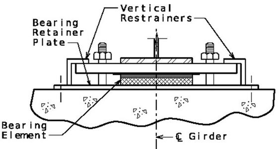 End Section thru Girder
 -
 Section thru Intermediate Bent Beam at Expansion Gap


Fig. 751.9.3.1.3.2 Examples of Vertical Restrainers

|
(1) (Expansion Gap @ 60°F) + 1/2“ |
Fig. 751.9.3.1.3.3 Longitudinal Restrainers (End Bents - Steel Girders)

|
Note: For skewed structures, see Figure 751.9.3.1.3.9.
|
Fig. 751.9.3.1.3.4 Longitudinal Restrainers (End Bents - Concrete Girders)

Note: For skewed structures, see Figure 751.9.3.1.3.9.
* Yb = Inches from bottom of beam, based on an 8½” slab.
| ||||||||||||||||||||||||||||||||||||||||||||||||||||||||||||||||
Fig. 751.9.3.1.3.5 Longitudinal Restrainers (Intermediate Bents - Concrete Girders)

|
(1) (Expansion Gap @ 60°F) + 1/2“ |
Fig. 751.9.3.1.3.6 Longitudinal Restrainers (Intermediate Bents - Steel to Concrete Girders)

|
(1) (Expansion Gap @ 60°F) + 1/2“ |
Fig. 751.9.3.1.3.7 Longitudinal Restrainers (Hinged Connection)

|
Note: Use Detail A for prestressed I-Girder structures at end and intermediate bents and also for all exterior
|
Fig. 751.9.3.1.3.8 Details A and B for Anchor Plates

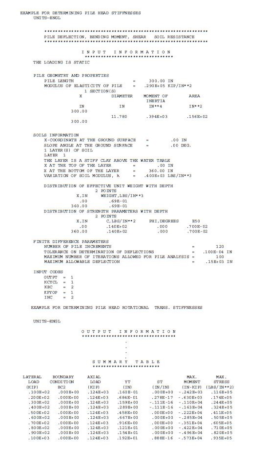
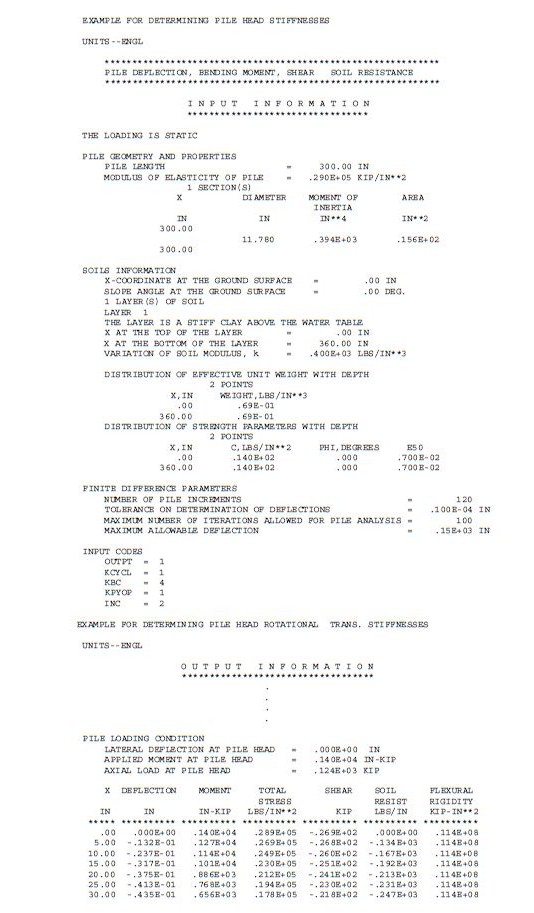
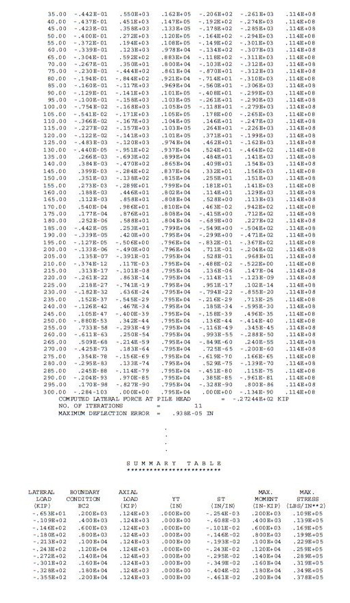
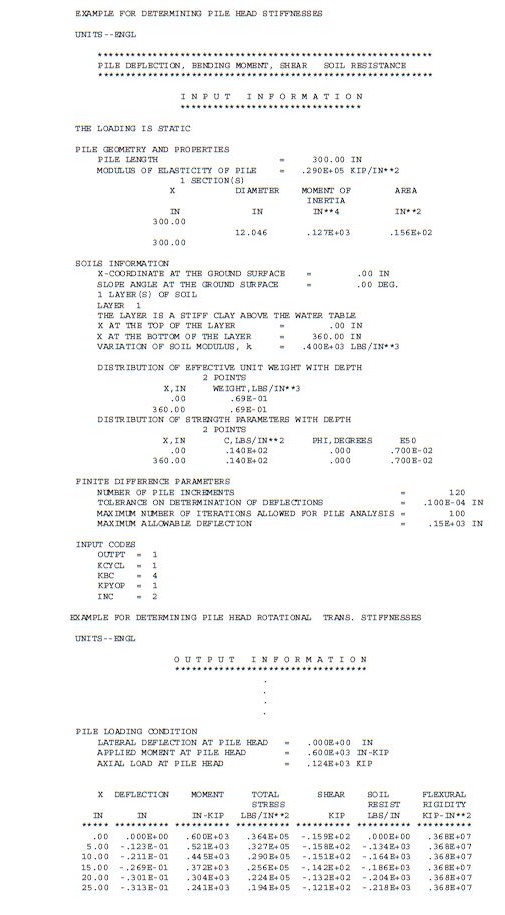
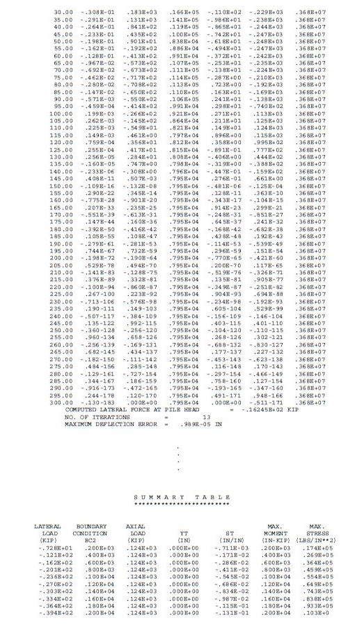
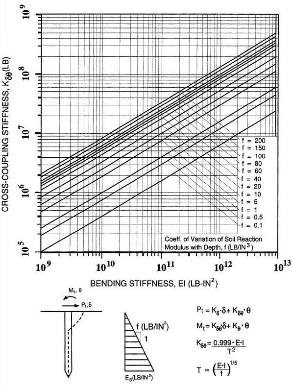
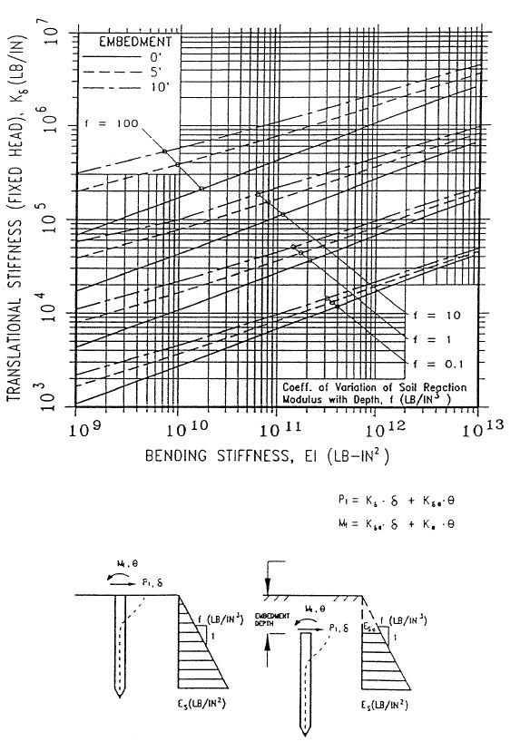
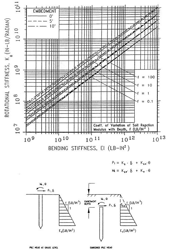
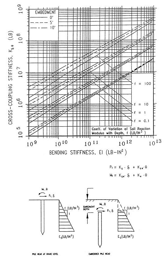
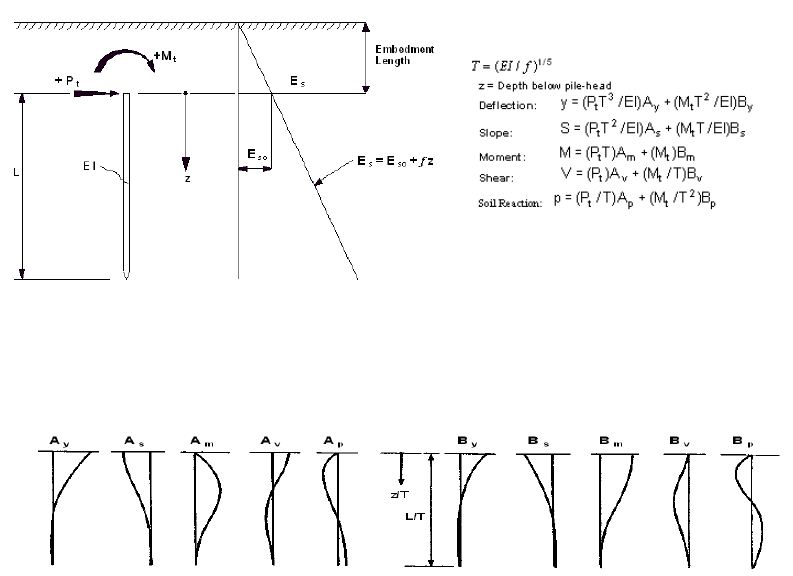
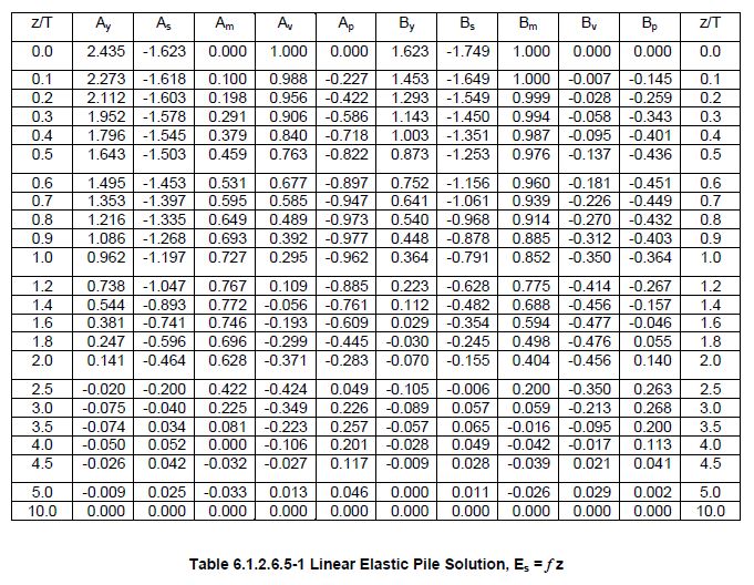
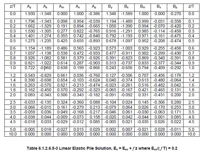
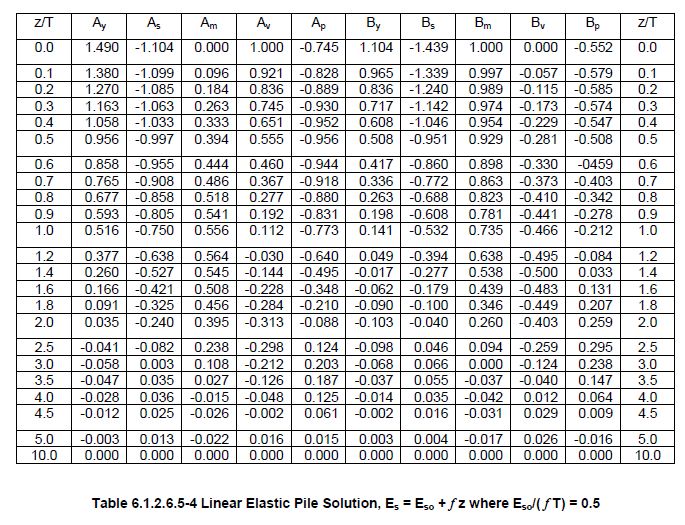
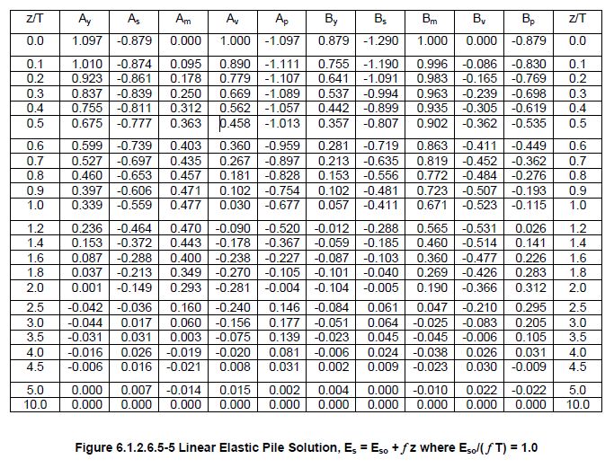
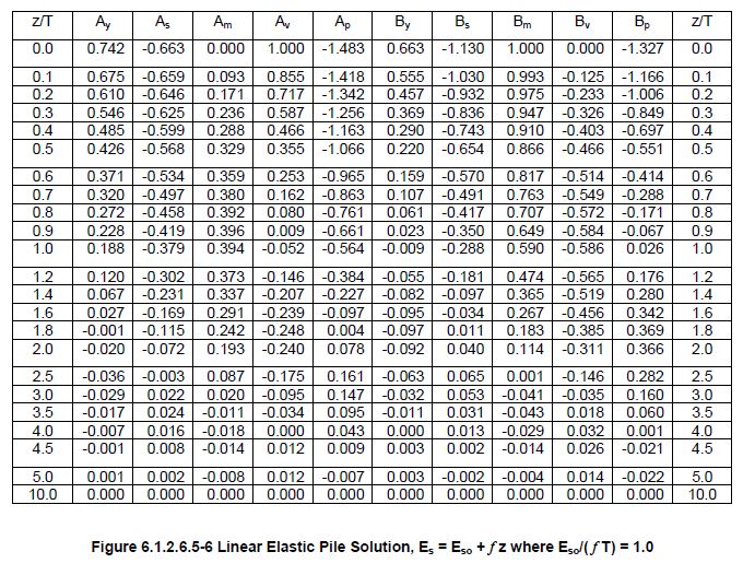
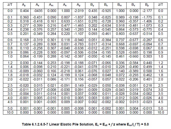
|
* For dimension properties of pipe, see AISC Steel Construction Manual, Part 1. |
Fig. 751.9.3.1.3.9 Details for Longitudinal Restrainers on Skewed Structures
751.9.3.1.4 Concrete Shear Blocks
For LRFD, see EPG 751.22.3.13 Concrete Shear Blocks for Concrete Shear Blocks design
751.9.3.1.5 Concrete End Diaphragms
Restrainers at Expansion Gaps, Concrete Girders
Design the concrete diaphragm thickness on P/S-I girder bridges with longitudinal restrainers at expansion gaps at abutments or intermediate bents. Check punching shear by Load Factor Design, as per AASHTO 8.16.6.6. Design force is the restrainer force used to size the rods in EPG 751.9.3.1.3. In tension, the failure surface is d/2 outside the outermost anchor studs.
751.9.3.1.6 Seismic Isolation Bearings
Isolation Bearings
Seismic isolation bearings shall conform to AASHTO Guide Specifications for Seismic Isolation Design, 3rd Ed., July 2010. Isolation bearings should only be used when specified on the design layout or when required for special retrofit projects. See the Structural Project Manager for approval and for the design specifications for the specific proprietary system to be used.
For LRFD, Seismic isolation bearings shall conform to AASHTO Guide Specifications for Seismic Isolation Design, 4th Ed., 2023.
751.9.3.1.7 T- Joint Connections for LFD
For LFD T-Joint connection requirement, see EPG 751.40.8.11.5 T- Joint Connections.
751.9.3.1.8 Anchorage of Piles for Seismic B, C and D
For anchorage of piles for seismic categories B, C and D, see EPG 751.36.4 Anchorage of Piles for Seismic Details.
751.9.3.2 Abutment Component Design
After Iterative Abutment Design has shown that abutment forces and displacements are acceptable, and after connection design is completed, the abutment components may be designed.
Wings (Integral OR Non-Integral Abutments)
- 1) Design the wing thickness for the applied shear on the wing. The design section is where the corner brace meets the inside edge of the wing. Use φ = 1.0 for shear. It is sometimes satisfactory to treat wing walls as fuse elements (i.e., broken off elements). This is mainly for integral abutment on very wide structures where large forces are drawn to the abutment. In this case, a second analysis with reduced stiffness in the transverse direction is required. Divide the wing up into two sections of f'c = 3 ksi and f'c = 4 ksi. Soil pressure acts below the bottom of the approach slab. See EPG 751.40 LFD Widening and Repair.
- 2) Design the flexural steel in the inside face of the wing (minimum #6 - H - bars @ 8" cts.) for the applied wing moment. Moment = (wing Area)*(soil pressure)*(arm from edge of corner brace to c.g. of wing area). The design section is where the corner brace meets the inside edge of the wing. Use φ = 1.0 for flexure. Divide the wing up into two sections of f'c = 3 ksi and f'c = 4 ksi. Soil pressure acts below the bottom of the approach slab. Position the wing reinforcement so that it does not interfere with girders or piles. The top of intermediate wings shall clear the bottom of the approach slab by a minimum of 3". See EPG 751.40 LFD Widening and Repair.
Non-Integral Abutments
- 3) For non-integral abutments, check the stability under application of active soil pressure. Find the Mononobe-Okabe (combined seismic and nonseismic) pressure and the Rankine (non-seismic) pressure. For the stability and reinforcement computations for non-integral Abutment Design, the height of the soil force resultant could be obtained by assuming that the non-seismic resultant force by Rankine theory acts at H/3 from the bottom of the backwall, while the seismic resultant force should be taken to act at a height of 0.6H. H is defined as the height of the backwall. See AASHTO Div. I-A Commentary for a description of Mononobe-Okabe active seismic soil pressure computations.
- 4) Design non-integral bent backwalls for shear due to soil pressure on the fill face of the backwall. The design section is at the base of the backwall, just above the beam. Use φ = 0.85 for shear, as in AASHTO 8.16.6.
- 5) Design non-integral bent backwalls for flexure due to soil pressure on the cantilevered backwall. The design section is at the base of the backwall, just above the beam. Use φ = 0.90 for flexure in AASHTO 8.16.3.
- 6) Design the backwall for flexure with the restrainers engaged (in tension) on the cantilevered backwall. In general, the soil pressure on the backwall can be neglected because it will be tensile when the restrainers are in tension, due to the separating motion of the superstructure. The design section is at the base of the backwall, just above the beam. Use φ = 0.90 for flexure in AASHTO 8.16.3.
- 7) Design the thickness of the backwall when restrainer anchor plates are present. For two-way shear (AASHTO 8.16.6), the design section is a rectangle surrounding the anchor plate. The design of anchor studs for restrainer anchor plates is described in EPG 751.9.3.1.3.
Deadman Anchors
- 8) Design deadman anchors, if present, as in EPG 751.40 LFD Widening and Repair.
751.9.3.3 Intermediate Bent Design
751.9.3.3.1 Column/Footing Intermediate Bents
Analysis
1) From dynamic analysis, determine seismic (EQ) force and moment demands at top and bottom of columns. These full elastic (R=1) forces assume elastic response under seismic loads.
2) Determine dead load demands (DL) at top and bottom of columns.
3) Calculate magnified moment due to full elastic, , and modified elastic, , moments (including minimum moment from eccentricity) at top and bottom of columns. Second-order effects shall also be considered.
Elastic Design, Without Plastic Hinging
4) Check the column (the size and reinforcement required for Groups I-VI is the minimum size column) using the full elastic (R=1) moments from Step (3) and φ = 0.75 to 0.9, as per AASHTO 8.16.1.2. Calculate 8 cases at 8 axial loads (P3max, P3min, P4max, P4min, at both top and bottom of each column):
- For LC 1.0*L + 0.3*T: a) P3max = DL + EQ, b) P3min = DL - EQ
- For LC 0.3*L + 1.0*T: a) P4max = DL + EQ, b) P4min = DL - EQ
If the column requires only a few bars to be designed elastically, then add a few bars rather than design the column for plastic hinging.
If UP/AP ≥ 1.0 (Ultimate moment over Applied resultant moment), then skip to Step (7) for no plastic hinging. Else, if UP/AP < 1.0, then perform Steps (5) and (6) first, considering plastic hinging.
Plastic Design, With Hinging
5) If UP/AP < 1.0 in Step (4), then determine the column size and reinforcement required for modified elastic (R=5) moments using φ = 0.5 to 0.9 as per AASHTO Div. I-A, Section 7.6.2(B). The column design required for Groups I-VI loads is the minimum size. Generate the column P-M interaction capacity curve. Plot the 8 combinations of axial and modified elastic moment on the same graph. If all the points lie within the curve, then the design is sufficient. If not, add bars and re-plot the curve until all points barely lie within the curve.
6) Determine the overstrength (φ = 1.3) plastic moment capacities of the column sized in step (5) as per AASHTO Div. I-A, Section 7.2.2. Use any non-linear push-over analysis program to determine the column overstrength moment, 1.3Mp, at the bent failure mechanism stage. If a non-linear pushover analysis program is not available, any static analysis program can be used by designating the hinging locations at top and/or bottom of column, use a joint release, then apply the overstrength plastic moment as a joint load.
Column Shear
7) Check column shear reinforcement (spirals) as required in AASHTO Div. I-A, Section 6.6.2 & 7.6.2, which specifies the required reinforcement ratio.
= ratio of volume of provided spiral reinforcement to total volume of concrete core, no units
As= cross-sectional area of one leg of spiral, sq. in.
Dc= diameter of spiral, out-to-out, inches
db= bar diameter of spiral, inches
Ac= area of core, out-to-out of spirals, sq. in.
s = spiral pitch or spacing, inches
For computation of shear demand, consider the possibility that hinging could occur between the top of the footing and the mud line, instead of at the column/footing junction. This situation could occur on footings with large overburdens and soils with high SPT blow counts, which could cause a shorter effective column length and a larger column shear demand.
Footing Design
8) Design footings under Load Factor Design with φ = 0.90 for flexure and φ= 0.85 for shear, as per AASHTO 8.16.1.2.
- Compare the moments from steps (4) and (6). If step (4) moments are lesser, then size the footings for the full elastic loads from step (4).
If step (6) moments are lesser, then size the footings for the overstrength plastic column moment capacities (Mop) from step (6) in all directions of possible hinging: a) In-plane hinging at its corresponding axial load, b) Outof-plane hinging at its corresponding axial load
- For spread footing pressure, keep resultants in the middle 2/3 of the footing.
- For the footing shear check, use Load Factor Design, with φ = 0.85.
- For footing reinforcement design, use Load Factor Design, with φ = 0.90. For spread footings, design top steel for weight of footing + weight of soil. For pile footings, design the top of footing reinforcement for weight of footing + weight of soil + seismic pile
tension. Check pile requirements in AASHTO Division I-A, Section 6.4.2 or 7.4.2.
Beam Design
9) Design beams under Load Factor Design, with φ = 0.90 for flexure and φ = 0.85 for shear, as per AASHTO 8.16.1.2.
- If the column design was OK (no hinging) under full elastic loads from Step (4), then consider dead loads and the seismic in-plane top-of-column shears and axial loads (for P-Δ effects) for the beam design.
- If the column design was controlled by modified elastic loads (with plastic hinging) from Step (5), then consider dead loads and the overstrength (φ = 1.3) plastic moments from Step (6) for the beam design. In this case, designate the hinging location as a support, use
a joint release, then apply the overstrength plastic moment as a joint load.
- For either elastic or plastic loads, design the beam for negative moments and for shear at faces of equivalent square columns, and design for maximum positive moments in between columns.
T-Joint Connection Design
10) Check the beam/column T-joint stresses and the column/footing T-joint stresses as described in EPG 751.9.3.1.7.
751.9.3.3.2 Pile Cap Intermediate Bents
Definitions of Terms
In AASHTO Div. I-A Sections 6 & 7, some AASHTO terms are different from MoDOT terms. AASHTO's "pile caps" are caps of pile footings or beam caps of pile bents, and are considered "foundations". AASHTO's "pile bents" are what MoDOT calls pile cap intermediate bents, and piles on pile bents are treated as columns, not as "foundations". MoDOT's CIP piles are considered in AASHTO both as "concrete-filled pipe piles" and as "Cast-in-Place concrete piles" with the shell considered as both longitudinal reinforcement and as shear reinforcement.
| Additional Information |
| AASHTO LRFD Specs., 5.10.11.4.1c&d&e, 5.13.4.5, 5.13.4.6 |
| AASHTO Division I, 4.5.17.4 |
For drilled shafts and piles, a plastic hinge developed above the ground line is allowed for trestle piles (at intermediate bents), but not for foundation piles (below the ground line). "Trestle" and "foundation" piles are as defined in EPG 751.40 LFD Widening and Repair.
Analysis of Bent
1) Model the bent according to EPG 751.9.2.8.1 or EPG 751.9.2.8.2.
2) From dynamic analysis, determine seismic (EQ) axial, moment and shear force demands of the piles. These full elastic (R=1) forces assume elastic response under seismic loads.
3) Determine dead load (DL) axial, moment and shear force demands of the piles.
Elastic Design, Without Hinging
4) The minimum pile size and reinforcement is that which was required for Groups I-VI. Check the minimum pile size using the full elastic (R=1) moments from Step (2) and φ = 0.75 to 0.9, as per AASHTO 8.16.1.2. Analyze the pile for axial / moment (P-M) interaction capacity for CIP piles. Steel piles are analyzed for buckling and for combined stresses as described in the AASHTO references.
| Additional Information |
| AASHTO Div. I-A,7.5.2 & AASHTO Div. I, 10.36 & 10.54 |
Analyze the pile at 4 axial loads (P3max, P3min, P4max, and P4min):
- For LC 1.0*L + 0.3*T: a) P3max = DL + EQ, b) P3min = DL - EQ
- For LC 0.3*L + 1.0*T: a) P4max = DL + EQ, b) P4min = DL - EQ
The shell of CIP piles provides shear reinforcement and longitudinal flexural reinforcement (see equations below). See EPG 751.40 LFD Widening and Repair for the design thickness of the shell.
If UP/AP ≥ 1.0, or if UP/AP ≥ 1.0 by adding only a few bars, then skip to Step (8) for no hinging. Else, if UP/AP < 1.0 or if it takes too many added bars to increase UP/AP to more than 1.0, then perform Steps (5) or (6) first, considering plastic hinging.
Plastic Design, With Hinging
5) If UP/AP < 1.0 for pile above the ground line in Step (4), then determine the pile size and reinforcement required for modified elastic (R=3 for vertical piles only and R=2 for one or more battered piles) moments using φ = 0.5 to 0.9 as described in AASHTO Div. IA, Section 7.6.2(B). The pile design required for Groups I-VI loads should be the minimum design. Generate the pile P-M interaction curve. For steel HP piles, combined stresses are computed as described in EPG 751.9.2.10.2. Plot the 4 points of axial and modified elastic moment on the same graph. If all the points lie within the curve, then the design is sufficient. If not, add bars or use a larger pile size, and re-plot the capacity curve until all points barely lie within the curve. Use R=1 to design pile under the ground line.
6) If a non-linear push-over analysis program is available, determine the plastic hinge locations based on the horizontal bent displacements from the seismic analysis. If any plastic hinges occurred below the ground line, redesign the bent by increasing the total number of pile or pile size, etc.
7) The end regions of concrete piles should be reinforced for plastic hinging. Refer to Fig. 751.9.3.3.2 for the following terms.
- A = the greater of (D/2 or 15")
- B = the greater of (2*D or H/6 or 24")
- D = the pile diameter, in inches
- G = A + B = the length of the upper plastic hinging region, in inches
- H = the pile clear height, from bottom of beam to mud line, inches

AASHTO Div. I-A, 7.6.2(D) specifies the reinforcement ratio required, and the provided reinforcement ratio is given by:
Shells of CIP Piles:
- Provided = the ratio of volume of reinforcement provided by
the shell to the total volume of the concrete core, no units.
- Where: t = Shell thickness
- D = Core Diameter
Spirals:
- Provided = the ratio of volume of reinforcement provided by the spiral to the total volume of the concrete core, no units.
- = cross-sectional area of one leg of spiral, sq. in.
- Where: DC= diameter of spiral, out-to-out, inches
- db= bar diameter of spiral, inches
- Ac= area of core, out-to-out of spirals, sq. in.
- s = spiral pitch or spacing, inches
Steel piles shall be provided with shear connector angles for anchorage.
| Additional Information |
| AASHTO Div. I-A, 7.4.2(C) & Bridge Manual Section 3.72, 4.6 & 5.5 |
Beam Design
8) Design beams under Load Factor Design, with φ = 0.90. If the pile design was OK (no hinging) under full elastic loads from Step (4), then consider dead loads and the seismic in-plane top-of-column shears and axial loads (for P-Δ effects) for the beam design. If the column design was controlled by modified elastic loads (hinging) from Steps (5) or (6), then apply dead loads and the overstrength (φ = 1.3) plastic moments from Steps (5) or (6). For either elastic or plastic loads, design the beam for the negative moments at faces of equivalent square piles and for the maximum positive moments in between piles. Check shear in the beam at the faces of the equivalent square piles. Minimum beam width shall be as per EPG 751.40 LFD Widening and Repair, but should also provide 6 in. concrete cover outside piles as per AASHTO Div. I Section 4.5.15.2. Note that for 20 in. and 24 in. CIP piles, the standard 30 in. integral end bent beam width must be enlarged to 32 in. and 36 in., respectively.
T-Joint Connection Design
9) Check the beam/pile T-joint stresses as described in EPG 751.3.1.7.
751.9.3.3.3 Drilled Shaft Intermediate Bents
Drilled shafts (also called "Pedestal Piles") are described in EPG 751.40 LFD Widening and Repair. In the following discussion, the portion of the pedestal pile above ground will be referred to as the "column". The portion of the pedestal pile below ground will be referred to as the "shaft". Most drilled shafts have a shaft diameter larger than the column diameter, as shown below in Fig. 751.9.3.3.3. Drilled shafts are drilled or augered in, whereas piles are driven into place.

The following discussion of drilled shafts assumes that the pile diameter is larger than the column diameter. The column portion is allowed to plastic hinge, but the shaft portion is not allowed to hinge.
Sometimes, there is an enlarged bell at the bottom when required for bearing pressure. EPG 751.40 Widening and Repair (Noon-LRFD) allows this bell only in SPC A, but unusual situations might require a bell in other Seismic Performance Categories. If a bell is required in SPC B, C or D, then reinforcement should be provided around the outside of the bell, in order to prevent local crushing of the bell.
Drilled shafts with no bell are socketed into rock a minimum distance of 1.5 times the shaft diameter and are considered fixed at the rock line. Drilled shafts with a bell are considered pinned at the rock line.
Analysis of Bent
1) Model the bent according to Sections 6.1.2.8.1 and 6.1.2.8.2.
2) From the dynamic analysis, determine seismic (EQ) axial, moment and shear force demands at "top of column" (near the beam/column joint) and at "bottom of column" (near the column/shaft joint). These full elastic (R=1) forces assume elastic response under seismic loads.
3) Determine dead load (DL) axial, moment and shear force demands at "top of column" and at "bottom of column".
4) Plastic hinging of the column portion of a drilled shaft is allowed for trestle piles (intermediate bents), but not for foundation piles (end bents), as defined in EPG 751.40 LFD Widening and Repair. The shaft portion of a drilled shaft is considered a "foundation" in AASHTO Div. I-A, 7.2.1(B), so plastic hinging of the shaft portion of a drilled shaft is not allowed. Calculate the full elastic moments at all tenth-points of the entire column & shaft, and calculate the modified elastic moments at tenth-points of the column portion.
Column Design, Without Hinging
5) Check the column portion and shaft portion (the minimum size and reinforcement is that which was required for Groups I-VI) using the full elastic (R=1) moments from Step 5 and φ = 0.75 to 0.9, as per AASHTO 8.16.1.2. Analyze the column and shaft for axial / moment (P-M) interaction capacity. Analyze the column at 8 axial loads (P3max, P3min, P4max, and P4min, top and bottom):
- For LC 1.0*L + 0.3*T, a) P3max = DL + EQ, b) P3min = DL - EQ
- For LC 0.3*L + 1.0*T, a) P4max = DL + EQ, b) P4min = DL - EQ
If UP/AP ≥ 1.0 or if UP/AP ≥ 1.0 by adding only a few bars, then skip to Step (8) for no hinging. Else, if UP/AP < 1.0 or if too many bars must be added, then perform Steps (6) and (7) first, for column plastic hinging.
Plastic Column Design, With Hinging
6) If UP/AP < 1.0 in Step (4), then the column portion is designed for modified elastic moments (R=5), and the shaft portion is designed as a foundation (R=1). Determine the column size and reinforcement required for modified elastic (R=5) moments using φ = 0.5 to 0.9 as described in AASHTO Div. I-A, Section 7.6.2(B), with the column design required for Groups I-VI loads as the minimum. Generate the column P-M interaction curve for drilled shafts. Plot the combinations (as in Step (5) above) of axial and modified elastic moment on the same graph for all 8 points on the column portion. If all the points lie within the curve, then the column design is sufficient. If not, add bars and re-plot the capacity curve until all points barely lie within the curve.
| Additional Information |
| AASHTO Div. I-A, 7.2.2(B), Step 2 |
7) The end regions of columns should be reinforced for plastic hinging. The end region length at either end of the column is the larger of (two times the column diameter, one-sixth of the clear height of the column, and 24 inches). The spiral at the bottom end of the column shall continue into the shaft for a distance equal to the greater of (half the column diameter or 15 inches).
Design column shear reinforcement (spirals) for the required reinforcement ratio described in the reference below.
| Additional Information |
| AASHTO Div. I-A, Section 7.4.2 & 7.6.2 |
For the provided reinforcement ratio of spirals:
- Provided = the ratio of volume of provided spiral reinforcement to total volume of concrete core, no units.
Where:
- As= cross-sectional area of one leg of spiral, sq. in.
- Dc= diameter of spiral, out-to-out, inches
- db= bar diameter of spiral, inches
- Ac= area of core, out-to-out of spirals, sq. in.
- s = spiral pitch or spacing, inches
Shaft Design
8) The design moments for the shaft shall be the lesser of the full elastic moments (R=1) from Step (5) and the overstrength plastic moment capacity (φ = 1.3) of the column sized in step (6).
| Additional Information |
| AASHTO Div. I-A, Section 7.2.1(B) & 7.2.2 & 7.2.6 |
Beam Design
9) Design the beam under Load Factor Design, with a flexural φ = 0.90 and a shear φ = 0.85. If the column design was OK (no hinging) under full elastic loads from Step (5), then apply dead loads and the seismic in-plane top-of-column shears and axial loads for the beam design. If the column design was controlled by modified elastic loads (hinging) from Step (6), then apply dead loads and the overstrength (φ = 1.3) plastic moments from Step (6). For either elastic or plastic loads, design the beam for the negative moments at faces of equivalent square columns and for the maximum positive moments in between columns. Check shear in beams according to hinging or no hinging.
T-Joint Connection Design
10) Check the beam/column T-joint stresses as described in EPG 751.9.3.1.7.
751.9.3.3.4 Integral Intermediate Bents
The difference between a standard intermediate bent and an integral intermediate bent is shown in Fig. 751.9.3.3.4.

On standard intermediate bents, the beam stirrups are completely contained within the beam, and a line of dowels creates only a "pinned" connection with the diaphragm and superstructure. Due to the roofing felt and the dowels, the "pinned" connection theoretically does not transfer moments between the superstructure and the substructure. A standard (non-integral) intermediate bent therefore exhibits single-curvature bending out of the plane of the bent. In-plane bending is double-curvature due to the moment connections between beam and columns or between beam and piles.
On an integral intermediate bent (non-standard), the beam stirrups extend up into the diaphragm (similar to standard integral end bents), making a "fixed" connection which can transfer moments between the superstructure and the substructure. This fixed connection makes the integral intermediate bent exhibit double-curvature bending out of the plane of the bent. In-plane bending is also double-curvature due to the moment connections between beam and columns or beam and piles.
When to Use Integral Intermediate Bents
1) When (KL)/R > 100 for piles or drilled shafts and a larger diameter member is not acceptable. This situation can be improved by making the intermediate bent integral, causing double-curvature out-of-plane bending (K = 1.2) instead of single-curvature out-of-plane bending (K = 2.0), thus reducing (KL)/R.
2) When the percentage of the total seismic force at the end bents is so high that other remedial actions are ineffective (see EPG 751.9.2.10). This situation can be improved by making the intermediate bents integral, which makes them stiffer and helps to distribute some of the excessive force from the end bents to the intermediate bents.
3) Sometimes, making the bent integral can help to stiffen up the entire bridge, decrease the period, and may improve the situation.
751.9.3.4 Cross Frame Analysis and Design
Recent earthquakes indicate that many steel bridges have suffered cross frame damage. Cross frames provide an important load path for the seismic force acting on slab-on-girder steel bridges. Cross frames shall be able to transmit all lateral forces from the superstructure to the bearings. The lateral seismic force at an individual bent calculated from the seismic analysis shall be proportionally distributed to the individual cross frames over the bent.
For details of cross frames, see EPG 751.40 LFD Widening and Repair. The components of cross frames including top and bottom chords and diagonal angle members shall be designed based on allowable stress design with consideration of the eccentric axial load and buckling stresses. Welding sizes at gusset plate connection shall also be designed for the seismic load. Cross frames shall remain elastic when subjected to the seismic force.
The following cross frame model may be used for the structural analysis of cross frames:

Study (S.M. Zahrai and M. Bruneau, 1999) has shown that bearing stiffeners provide the main stiffness for girders; in other words, using a longer length of girder (greater than 20 inches) in the model in Fig. 751.9.3.4.1 results in no significant difference in model stiffness. Based on the cross frame model in Fig. 751.9.3.4.1, the following structural analysis model can be considered:

In Fig. 751.9.3.4.2, Iy = moment of inertia of the stiffened stub girder (mainly due to the bearing stiffeners) in the lateral direction (i.e. y-y direction). The above model assumes full fixity at the concrete deck and zero fixity at the flexible bearings such as elastomeric bearings.
751.9.4 References
Cheney, R.S., and Chassie, R.G. (1982), “Soils and Foundation Workshop Manual,” U.S. Department of Transportation, Federal Highway Administration.
FHWA, “ Seismic Retrofitting Manual for Highway Bridges,” FHWA-RD-94-052, May 1995.
Kavazanjian, E. Jr., Matasovic, N., Hadj-Hamou, T., and Sabatini, P.J., “Geotechnical Engineering Circular No. 3, Design Guidance: Geotechnical Earthquake Engineering for Highways,” Volume 1- Design Principles, FHWASA- 97-076, 1997.
Lam, I.P., Kapnskan, M., and Chandhuri, D., “Modeling of Pile Footings and Drilled Shafts for Seismic Design,” MCEER Report 98-0018, 1998.
Lam, I.P., and Martin, G.R., “Seismic Design of Highway Bridge Foundations,” Federal Highway Adminstration Report # RD-86-101, 102, 103, 1986.
Lambe, T.W., and Whitman, R.V. (1969), Soil Mechanics, John Wiley and Sons, Inc., New York.
Meyerhof, G.G.(1976), “Bearing Capacity and Settlement of Pile Foundations,” Journal of Geotechnical Engineering Division, ASCE, Volume 102, No. GT3, Proc. Paper 11962.
NHI Course No. 13063, “Seismic Bridge Design Applications,” Session 6, 1996.
Norlund, R.L. (1963), “Bearing Capacity of Piles in Cohesionless Soils,” ASCE, SM&F Journal SM-3.
Norlund, R.L. (1979), “Point Bearing and Shaft Friction of Piles in Sand,” 5th Annual Fundamentals of Deep Foundation Design, University of Missouri-Rolla.
Priestley, M.J.N., and Seible, F., (1996) Seismic Design and Retrofit of Bridges, John Wiley and Sons.
Thurman, A.G. (1964), “Computed Load Capacity and Movement of Friction and End-Bearing Piles Embedded in Uniform Stratified Soil,” Ph.D. Thesis, Carnegie Institute of Technology.
Tomlinson, M.J. (1985), “Foundation Design and Construction,” Longman Scientific and Technical, Essex, England.
United States Steel (1965), Highway Structures Design Handbook, Volume 1, Chapter 10.
Urzua, A. (1993), SPILE: A Microcomputer Program for Determining Ultimate Vertical Static Pile Capacity, User’s Manual, FHWA-SA-92-044.
Wang, S.C., and Reese, L.C. (1993), COM624P- Laterally Loaded Pile Analysis Program for the Microcomputer, FHWA-SA-91-048.
Wilson, J.C. (1988), Stiffness of Non-Skew Monlithic Bridge Abutments for Seismic Analysis, Journal of Earthquake Engineering and Structural Dynamics Vol. 16.
Zahrai, S.M., and Bruneau, M. (1999) Ductile End-Diaphragms for Seismic Retrofit of Slab-on-Girder Steel Bridges, Journal of Structural Engineering, ASCE, Volume 125, No. 1.